8 Index Tracking

8.1 Learning Objectives
After completing this chapter, you will be able to …
explain the key concepts and goals of index tracking and clearly distinguish them from active portfolio strategies, particularly in terms of costs, risk, and deviations from the reference index.
compute and interpret the tracking error—the central metric in index tracking—and use it to assess how well an index-replication strategy performs.
describe and compare the various index-tracking approaches and analyze their respective strengths and weaknesses.
formulate an index-tracking problem as an optimization task, specify appropriate constraints, and give an economic interpretation of the resulting portfolio weights.
implement an index-tracking strategy in Python using the relevant libraries and critically assess the results in terms of replication accuracy, stability, and practical usability.
8.2 Introduction and motivation
The following discussion draws on Chapter 4 of Poddig et al. (2009).
The term “index tracking” refers to replicating a given target portfolio with a portfolio that is actually held or implemented (tracking portfolio). The target portfolio may be a benchmark portfolio—for example, a market index for a particular securities market. The aim is to construct the tracking portfolio so that its performance matches that of the target portfolio as closely as possible.
The motivations for index tracking fall broadly into two groups: (1) reasons rooted in the investment philosophy and stance of the (portfolio) management or arising from specific trading strategies, and (2) reasons that are more “technical” in nature.
The first group rests on the distinction between active and passive portfolio management. Constructing portfolios through absolute and relative optimization assumes that capital markets are information-inefficient and that the manager believes in their own, presumably superior, forecasting ability. Such a manager is convinced that they can forecast future market developments well enough that the systematic (risk-adjusted) excess return of the resulting active portfolio outweighs the costs of gathering and evaluating information and of active management. If one’s forecasting ability is inadequate, or if the entire active-management process proves too costly relative to the excess returns it can achieve, it should be abandoned—and the task then becomes simply to implement the given benchmark portfolio as cost-effectively as possible.
Specific trading strategies may also call for replicating an index; examples include trading or issuing index products and derivatives, and certain arbitrage strategies that rely on index portfolios.
The “technical” reasons for index tracking can be highly varied and may, of course, also arise alongside a deliberate choice of passive management or the use of specific trading strategies. They come down essentially to two causes: acquiring the target portfolio, or parts of it, is (1) impossible or impermissible, or (2) too expensive. The target portfolio may, for instance, be a synthetic (capital-market) index—a fictitious securities portfolio that cannot be purchased. Alternatively, certain target-portfolio assets may not be available, or not to the extent required, because of legal, statutory, or mandate-related restrictions.
8.3 Constructing tracking portfolios
8.3.1 Overview
There are many ways to replicate a target portfolio (a benchmark portfolio, market index, etc.). The most obvious is full replication: every asset in the target portfolio is held in the tracking portfolio at the same weight. By construction, this reproduces the target portfolio exactly, but for the reasons noted above (high costs, among others) it is rarely feasible in practice. This creates the need for approximate replication (sampling), in which the tracking portfolio’s composition may differ (sometimes substantially) from the target portfolio while still tracking its performance as closely as possible. The basic approaches are either heuristic (stratified sampling) or optimization-based (optimizing sampling). Stratified sampling is not covered here, as it lacks a theoretical foundation; the following discussion is devoted to optimizing sampling. We present quadratic optimization, data-analysis, and linear optimization procedures in turn.
8.3.2 Quadratic optimization procedures
8.3.2.1 Relative optimization and index tracking
The following shows how the relative-optimization procedure can be repurposed, with only minor modifications, to determine the structure of an “optimal” tracking portfolio.
Constructing a tracking portfolio can be characterized by two points:
A target portfolio (benchmark, index, etc.) is given, whose performance and risk are to be tracked (replicated) as accurately as possible by a tracking portfolio that has yet to be determined.
For various reasons, the tracking portfolio may have to be built from assets not contained in the target portfolio. Conversely, not all assets in the target portfolio may be available for the tracking portfolio, or their weights in it may be restricted. The investment universes and constraints of the target and tracking portfolios can therefore differ considerably.
This problem structure clearly resembles that of relative optimization with different investment universes. Here, however, the goal is not to maximize portfolio alpha against residual (active) risk, since the objective of relative optimization does not fit the objective pursued here.
This raises the question of when the benchmark portfolio is replicated “as well as possible.” Intuitively, the tracking portfolio must have the following properties:
- Its alpha (relative to the benchmark, i.e. the target portfolio) must be zero (since the benchmark alpha is zero).
- Its beta must be one (since the benchmark beta is one).
- Its residual (= active) risk must be minimal.
The target function follows from the goal of tracking the benchmark as closely as possible. This amounts to minimizing the active risk \(\sigma^2_{AP}\), which, once the timing component is excluded (i.e. \(\beta_P=1\)), reduces to the residual risk \(\sigma^2_{\epsilon_P}\). The target function is therefore:
\[ \begin{split} \\(1a) \quad TF(w) = \sigma^2_{\epsilon_P} \rightarrow \min_{w}!, \\ \end{split} \]
or, in matrix notation, using the relationship \((\sigma^2_{\epsilon_P}=\sigma^2_P-\beta^2_P*\sigma^2_B)\):
\[ (1b) \quad TF(w) = w_P^T\Sigma w_P-(w_P^T\beta)^2*w_B^T\Sigma w_B \rightarrow \min_{w}! \]
The main constraints are the same as in relative optimization:
\[ \begin{split} & \text{(a)}\ w^{T}\iota = 1 \quad or \quad \ w_A^{T}\iota = 0 \qquad \text{(budget constraint)}, \\ & \text{(b)}\ w\geqq 0 \qquad \text{(long-only constraint)}, \\ & \text{(c)}\ \beta_P=1 \quad \Leftrightarrow \quad \beta_{AP}=0 \quad \text{(no timing)}. \end{split} \]
To replicate the benchmark portfolio in its key properties, we must require, in addition to a portfolio beta \(\beta_P\) of one, a portfolio alpha \(\alpha_P\) of zero:
\[ \begin{split} & \text{(d)}\quad \alpha_P=0 \quad \text{(no selection)}. \end{split} \]
Because the tracking portfolio must be assembled from assets other than the benchmark itself, a selection effect arises unintentionally but unavoidably. Constraint (d) ensures that no systematic selection effect—a positive or negative portfolio alpha—occurs, but temporary (unsystematic) deviations between the tracking-portfolio return and the benchmark return are inevitable. Under the given constraints, these deviations show up as an unavoidable selection risk, which here coincides with the unavoidable “active” risk. This risk should be as small as possible, so the portfolio we seek is the one with the smallest possible unavoidable selection risk (= active risk).
8.3.2.2 Deriving the tracking error (TE)
To the extent that the tracking portfolio does not exactly match the benchmark portfolio, a return difference (= active return) between the two can arise:
\[ (2) \quad r_A=r_P-r_B \]
where
- \(r_{A}\) : active return
- \(r_{P}\) : return of the tracking portfolio
- \(r_{B}\) : return of the benchmark portfolio.
Assuming a univariate linear return-generating process with the target portfolio as the benchmark, the tracking-portfolio return satisfies:
\[ (3) \quad r_P=\alpha_P + \beta_P*r_B+\epsilon_P, \]
where:
- \(\alpha_P\): the portfolio \(P\)’s autonomous return (constant)
- \(\beta_P\): sensitivity to the benchmark portfolio \(B\)
- \(\epsilon_P\): the unsystematic, random, unexplained residual term.
Using constraints (c) and (d), the active return follows as:
\[ (4) \quad r_A=r_P-r_B=\alpha_P + \beta_P*r_B+\epsilon_P-r_B=\alpha_P+\epsilon_P=\epsilon_P. \]
Under the standard assumptions of a return-generating process, the expected active return is:
\[ (5) \quad E(r_A)=E(\epsilon_P)=0. \]
In index tracking, the variance (or, alternatively, the standard deviation) of the active return is known as the tracking error (TE):
\[ (6a) \quad TE=Var(r_A)= Var(r_P-r_B) \quad or \\ (6b) \quad TE=\sqrt{(Var(r_A))}=\sqrt{Var(r_P-r_B)} \]
Since the variance of a random variable \(X\) is \(Var(X)=E(X^2)-E(X)^2\), equation (6a) can be rewritten as equation (7):
\[ (7) \quad Var(r_P-r_B)= E((r_P-r_B)^2)-E(r_P-r_B)^2 \\ \quad = E((r_P-r_B)^2)-E(\epsilon_P)^2=E((r_P-r_B)^2). \]
As shown in the chapter on relative optimization, the risk attributable to the active position—the active risk—can also be defined via equation (8):
\[ (8) \quad \sigma^2_{AP}=w^T_A\Sigma w_A=Var(r_A) \]
where \(w_A\) is the column vector of the tracking portfolio’s active weights \((w_A=w_P-w_B)\). In index tracking, equation (8) therefore also represents the tracking error—that is, the “active” variance of the tracking portfolio. Following equation (2) in the “Active beta” section on relative optimization, we also have:
\[ (9) \quad TE=\sigma^2_{AP}=\beta^2_{AP}\sigma^2_B + \sigma^2_{\epsilon_P} \]
Because of constraint (c), equation (9) simplifies in this approach to equation (10).
\[ (10) \quad TE=\sigma^2_{AP}= \sigma^2_{\epsilon_P} \]
With the target function in equation (1), this approach therefore minimizes the tracking error, which is the usual way of determining a tracking portfolio. Using the relationship derived in equation (7), we further have:
\[ (10) \quad TE=\sigma^2_{AP}= \sigma^2_{\epsilon_P}=E((r_P-r_B)^2). \]
The target function in equation (1) can thus also be written as equation (11):
\[ (11) \quad TF(w)= E((r_P-r_B)^2) \rightarrow \min_{w}! \]
This clarifies the meaning of the target function in equation (1): minimizing it is equivalent to minimizing the expected squared return difference between the tracking portfolio and the benchmark. In other words, what is minimized here is the (expected) mean squared error between the two return series.
Procedurally, then, determining a tracking portfolio can be understood as a special case of relative optimization with different investment universes—requiring only a modified target function and the addition of constraint (d).
8.3.2.3 Index tracking according to Markowitz (1987)
Here, too, we start from a tracking portfolio that must (necessarily) differ in composition from the target portfolio, since the investment universes may differ and, for cost reasons, the tracking portfolio is generally built from far fewer assets than the target portfolio contains. The tracking portfolio must therefore be treated like an active portfolio: it unavoidably has an active return and an active risk. An ideal tracking portfolio has zero active return and zero active risk.
The active position is defined as the difference in weights between the held (tracking) portfolio \(P\) and the target portfolio \(B\), which we equate with the benchmark portfolio:
\[ (1) \quad w_A= w_P-w_B \]
The expected active return (bonus return) is the expected return difference between the (tracking) portfolio \(P\) and the benchmark \(B\) (the target portfolio):
\[ (2) \quad \mu_A= \mu_P-\mu_B=w^T_P \mu - w^T_B \mu = (w^T_P-w^T_B) \mu = w^T_A \mu \]
where \(\quad \mu : \quad\) is the column vector of expected asset returns.
The active risk (active variance) is:
\[ (3) \quad Var(r_A)=\sigma^2_{AP}=w^T_A \Sigma w_A. \]
This is also the usual definition of the tracking error (cf. equation (8) above):
\[ (4) \quad TE=Var(r_A) =Var(r_P-r_B). \]
The optimization now consists in minimizing the tracking error subject to various constraints. The target function is thus:
\[ (5) \quad TF(w)= TE= Var(r_A)=\sigma^2_{AP}=w^T_A \Sigma w_A \rightarrow \min_{w}! \]
The central constraint requires the expected active return to equal a target level \(\mu^*\), which is usually set to \(\mu^*=0\):
\[ (6) \quad \mu_A=w^T_A \mu = \mu^* (=0, usually) \]
The remaining constraints concern the budget constraint, the long-only constraint on the weights (where short selling is excluded), any required and permissible minimum and maximum weight limits, and, where appropriate, any other reasonable restrictions.
In practice, constraint (6) is often dropped. This has two apparent advantages: it simplifies the optimization problem, and it removes the need to estimate expected returns (precisely what index tracking aims to avoid). The downside is that the solution may then have a negative expected active return.
8.3.2.4 Comparison of the two approaches
The Markowitz approach has the apparent advantage of requiring only a few, comparatively unproblematic, quantities to be estimated. If constraint (6) is dropped when determining the tracking portfolio, only the future variance-covariance matrix needs to be estimated. This can be done with the empirical variance-covariance matrix, which in most cases provides “usable” estimates. The critical and very difficult estimation of the expected asset returns (the vector \(\mu\)) is avoided entirely. In this sense, the approach gets by with few input parameters that tend to be relatively uncritical and easy to estimate.
By contrast, index tracking based on relative optimization additionally requires the more elaborate and more critical estimation of the individual assets’ alpha and beta parameters. At first glance, this exposes it far more to the problem of estimating future quantities.
But the Markowitz approach escapes this additional estimation problem only because it simply ignores it! Without constraint (6), there is nothing to rule out that
- the tracking portfolio has a negative (expected) active return, and
- its beta departs from one, i.e. it exhibits an unwanted timing component.
To control these two effects, constraint (6) must be reinstated and the expected asset returns must be estimated after all. Seen this way, the two approaches are ultimately equivalent with respect to the estimation problem they face.
8.3.3 Regression subject to constraints
This procedure can be cast as a regression problem. The idea is to explain the benchmark returns \(r_{Bt}\) observed over a past period \(t=1, ..., T\) (the dependent variable in a multivariate linear least-squares regression) using the returns \(r_{it}\) of \(N\) assets (the independent variables). For an arbitrary point in time \(t\), we then require:
\[ (1) \quad r_{Bt}=w_{P1}r_{1t}+w_{P2}r_{2t}+...+w_{PN}r_{Nt}+\epsilon_t. \]
Here the (regression) residual \(\epsilon_t\) is the unsystematic, unexplained, random component relative to the benchmark return. The “tracking error” (return difference, active return) \(\epsilon_t\) is obtained by simply rearranging equation (1). The sum on the right-hand side of equation (1)—the bracketed expression in equation (2)—is clearly the return of the tracking portfolio:
\[ (2) \quad \epsilon_t=r_{Bt}-(w_{P1}r_{1t}+w_{P2}r_{2t}+...+w_{PN}r_{Nt}). \]
The “optimal” tracking portfolio has the smallest “tracking error” over the \(T\) periods and therefore satisfies:
\[ (3) \quad \Sigma^T_{t=1}\epsilon^2_t=\Sigma^T_{t=1}(r_{Bt}-(w_{P1}r_{1t}+w_{P2}r_{2t}+...+w_{PN}r_{Nt}))^2 \rightarrow \min_{w}!\ \]
Strictly speaking, equation (3) states an ex post requirement on the optimal tracking portfolio, while the unknown weights \(w_{Pi}\) are estimated from ex ante observations. This rests on the key assumption that the relationships observed in the past (the distribution of the benchmark and asset returns) will continue to hold in the future. The full target function to be minimized is therefore:
\[ (4) \quad TF(w)=\Sigma^T_{t=1}\epsilon^2_t=\Sigma^T_{t=1}(r_{Bt}-(w_{P1}r_{1t}+w_{P2}r_{2t}+...+w_{PN}r_{Nt}))^2 \rightarrow \min_{w}!\ \]
Comparison with the quadratic optimization procedures
Although the target function in equation (4) is closely related in substance to the previous approaches, the estimation technique is entirely different. On closer inspection, the two quadratic optimization procedures above determine the tracking portfolio in two separate steps:
- Estimating the input parameters needed for the optimization: depending on the procedure and its level of detail, this means estimating the variance-covariance matrix \(\Sigma\), the expected-return vector \(\mu\), or the alpha and beta values. These estimates may—but need not—be based on (simple) historical estimation; they can also be produced by entirely different procedures.
- Determining the tracking portfolio by optimizing an target function based on the input parameters from step 1.
The regression approach, by contrast, dispenses with the two-stage procedure and determines the tracking portfolio directly, in a single step, via a least-squares regression subject to constraints. Its advantage is procedural simplicity: it avoids the cumbersome intermediate step of estimating the required input parameters. Yet this is also the source of its key drawback—it cannot accommodate estimation procedures better than simple historical estimation. The quadratic optimization approaches are far more flexible here: better estimation procedures for the input parameters can be swapped in at any time without changing the overall approach, which is a substantial advantage.
8.3.4 Linear optimization
In the regression approach of the previous section, the return of the target portfolio (the benchmark portfolio \(B\)) is replicated as closely as possible at arbitrary (future) points in time \(t\) using \(N\) assets, leaving an unavoidable residual error \(\epsilon_t\). The unknowns to be determined are the weights \(w_{Pi}\) of the \(N\) assets in the tracking portfolio:
\[ (1) \quad r_{Bt}=w_{P1}r_{1t}+w_{P2}r_{2t}+...+w_{PN}r_{Nt}+\epsilon_t. \]
Whereas the earlier approaches aim, ideally, to drive the residual errors to \(\epsilon_t=0\) at all (future) points in time \(t\), here we take a different route. The active return \(r_A\) is the difference between the portfolio return and the benchmark return. Defining the residual error \(u_t=-\epsilon_t\), equation (1) can be rewritten as equation (2):
\[ (2) \quad r_{At}=r_{Pt}-r_{Bt}=u_t. \]
Naturally, an investor cares about not falling short of the benchmark return with the tracking portfolio and will therefore want to avoid \(u_t<0\). Positive deviations from the benchmark, i.e. \(u_t>0\), are by contrast quite welcome. On this view, the ideal tracking portfolio minimizes the sum of the absolute values of all negative active returns (residual errors \(u_t\)): it minimizes the investor’s expected shortfalls while preserving all upside potential. The target function for determining the tracking portfolio is thus:
\[ (3) \quad TF(w)=\Sigma^T_{t=1\\r_{Pt}<r_{Bt}} |r_{Pt}-r_{Bt}| \rightarrow \min_{w}! \]
The basic idea, then, is to determine the tracking portfolio so as to minimize the sum of the absolute (future) negative return deviations from the benchmark. This rests on a one-sided notion of risk: only shortfalls below the benchmark return count as undesirable outcomes to be avoided.
Strictly speaking, the target function in equation (3) again refers to the future and thus involves ex post quantities. To optimize the tracking portfolio, it must be estimated, usually from \(T\) past observation periods of the benchmark and asset returns (historically based estimation).
8.3.4.1 Implementing the target function via the auxiliary variables \(d^+_t\) and \(d^-_t\)
We introduce two auxiliary variables. Let \(d^+_t\) denote, as a positive number, the amount by which the tracking-portfolio return exceeds the benchmark return; conversely, let \(d^-_t\) denote, also as a positive number, the amount by which it falls below the benchmark. Using these two variables, the active return \(r_{At}\) (the residual error \(u_t\)) can be written as
\[ (4) \quad r_{At}=u_t=d^+_t-d^-_t \]
where
\[ (5a) \quad d^+_t=r_{Pt}-r_{Bt}, \quad \text{if} \quad r_{Pt}>r_{Bt} \\ d^+_t=0 \quad \text{otherwise} \]
\[ (5b) \quad d^-_t=r_{Bt}-r_{Pt}, \quad \text{if} \quad r_{Pt}<r_{Bt} \\ d^-_t=0 \quad \text{otherwise}. \]
By definition, \(d^+_t \geq 0\) and \(d^-_t \geq 0\). Moreover, \(d^+_t>0\) immediately implies \(d^-_t=0\), and conversely \(d^-_t>0\) implies \(d^+_t=0\). Substituting equation (4) into equation (2), equation (6) therefore holds at each point in time \(t\):
\[ (6) \quad r_{Pt}-r_{Bt}=d^+_t-d^-_t. \]
Equations (7a) and (7b) are equivalent to equation (6) and also hold at each point in time \(t\):
\[ (7a) \quad r_{Pt}-r_{Bt}-d^+_t+d^-_t=0 \quad or \\ (7b) \quad r_{Pt}-d^+_t+d^-_t=r_{Bt}.\]
Substituting the known expression \(\Sigma^N_{i=1} w_{Pi}r_{it}\) for the tracking-portfolio return in (7b) yields variant (7c):
\[ (7c) \quad \Sigma^N_{i=1} w_{Pi}r_{it}-d^+_t+d^-_t=r_{Bt} . \]
Using the auxiliary variables, the target function to be minimized in equation (3) can be rewritten as equation (8):
\[ (8) \quad TF=\Sigma^T_{t=1} d^-_t \rightarrow \min! \]
The optimization determines the following unknowns:
- the \(N\) asset weights \(w_{Pi}\),
- the \(T\) positive return deviations \(d^+_t\) (i.e. the positive active returns \(r_{At}\), or positive residual errors \(u_t\)), and
- the \(T\) negative return deviations \(d^-_t\) (i.e. the negative active returns \(r_{At}\), or negative residual errors \(u_t\)),
that is, \(N+T+T\) problem variables in all. The idea is to determine the weights \((w_{Pi})\) and the residual errors \((d^+_t-d^-_t)\) jointly so that
- in every period \(t=1, ..., T\), the tracking-portfolio return minus the residual error equals the benchmark return—i.e. equation (7c) holds for all \(T\) periods—and
- the sum of the negative residual errors \(d^-_t\) is thereby minimized.
In summary, the optimization for determining the tracking portfolio reads:
\[ (9) \quad TF=\Sigma^T_{t=1} d^-_t \rightarrow \min! \]
The main constraints are:
\[ \begin{split} & \text{(10)}\quad \Sigma^N_{i=1} w_{Pi}r_{it}-d^+_t+d^-_t=r_{Bt} \qquad \text{for all points in time} \space t=1, ..., T \\ & \text{(11a)}\quad d^+_t \geq0 \qquad \text{for all points in time} \space t=1, ..., T \\ & \text{(11b)}\quad d^-_t \geq0 \qquad \text{for all points in time} \space t=1, ..., T. \\ \end{split} \]
To these are added the usual constraints: the budget constraint, the ban on short selling, and possibly further restrictions such as required minimum weights and permissible maximum weights for the assets in the tracking portfolio.
This approach, too, faces an estimation problem. The target function actually to be minimized in equation (3) involves ex post quantities and, to determine a concrete tracking portfolio, is estimated via its ex ante formulation, i.e. from past observations. The quality of this ex ante estimation is therefore decisive for whether the tracking portfolio later lives up to expectations. Another aspect of the estimation problem is the number of unknowns in this approach. Besides the \(N\) tracking-portfolio weights \(w_{Pi}\) that are actually of interest, the optimization must also determine the \(T\) values each of the auxiliary variables \(d^+_t\) and \(d^-_t\)—together \(N+2T\) free parameters. If, say, 30 assets are considered for the tracking portfolio and the target function is estimated over 240 months of monthly returns, this gives 510 free parameters to be determined in the optimization. Since the problem is linear, however, this is generally not an issue.
8.3.5 The estimation problem of the optimization parameters
A key motive for passive portfolio management is the conviction that one lacks forecasting ability good enough to generate sufficient systematic excess returns through active management. Forecasts (estimates of future quantities) are therefore dispensed with, and the given benchmark is tracked with a tracking portfolio.
A closer look at the procedures for determining tracking portfolios reveals, however, that as soon as passive management turns to approximate replication (sampling) of the benchmark, it faces the same forecasting problem as active management. So what is gained?
The estimation problem tends to matter less for a tracking portfolio that
- shares the benchmark’s investment universe,
- contains many assets, and
- stays close to the benchmark in its weights,
than for a tracking portfolio that
- is (or must be) built from a different investment universe,
- contains rather few assets, and
- therefore departs substantially from the benchmark’s structure in both its constituents and their weights.
8.4 Case study
We begin by importing the required packages.
8.4.1 Loading and describing the dataset
The dataset contains price histories for the following ten stocks: Danone, Siemens, BASF, L’Oreal, Allianz, Telecom Italia, Banco Santander, Total, BMW, and Vivendi. The price history of the Euro Stoxx 50 index is included as the eleventh column.
The task of the case study is thus to construct, from the ten individual securities, the optimal tracking portfolio for the target portfolio—the Euro Stoxx 50.
The data consist of 111 monthly closing prices (“Adjusted Close”) covering the period from 31 December 2002 to 28 February 2012.
| Danone | Siemens | BASF | L'Oreal | Allianz | Telecom Italia | Banco Santander | Total | BMW | Vivendi | EuroStoxx 50 | |
|---|---|---|---|---|---|---|---|---|---|---|---|
| 2002-12-31 | 30.2427 | 40.50 | 18.040 | 72.55 | 82.025 | 2.0558 | 5.8537 | 33.5794 | 28.92 | 15.39 | 2386.41 |
| 2003-01-31 | 27.6478 | 38.15 | 17.260 | 64.30 | 66.860 | 2.0199 | 5.1466 | 30.9888 | 27.26 | 15.64 | 2248.17 |
| 2003-02-28 | 25.9021 | 36.78 | 16.910 | 59.90 | 60.137 | 1.8927 | 5.3256 | 30.2486 | 26.00 | 13.02 | 2140.73 |
| 2003-03-31 | 27.2939 | 37.80 | 17.055 | 55.50 | 41.080 | 2.0074 | 5.2361 | 28.6202 | 25.44 | 12.18 | 2036.86 |
8.4.2 Relative optimization and index tracking
The basic procedure is that of relative optimization with different investment universes. From the excess returns, we estimate the vector of future expected asset returns \(\mu\) and the future variance-covariance matrix \(\Sigma\) using historically based estimation.
Note: In the index-tracking procedures discussed above, it does not matter whether one starts from absolute or excess returns; what matters is that they be used consistently.
Estimation vs. validation period: The data comprise 111 monthly observations of prices or index levels, from which 110 (discrete) monthly returns can be computed for the individual securities and the index. To illustrate the importance of the estimation problem, the data are split into an estimation period (the first 60 monthly returns) and a validation period (the last 50). The tracking portfolios are always determined from the first 60 observations (the estimation period). Once a tracking portfolio has been determined, we then compute, over the validation period, the (mean) active return and its variance (the tracking error) that the portfolio would have realized. With perfect estimates of the input parameters, the estimated ex ante tracking error (from the estimation period) should ideally roughly match the actual, ex post tracking error of the validation period. A single case study cannot support general conclusions about the quality of the individual procedures, but it can nonetheless illustrate the underlying problem.
Code
# calculation based on discrete returns
returns = frame.pct_change().dropna()

rf = (1+0.04)**(1/12)-1 # risk-free rate assumed 4% p.a.
ex_returns = returns - rf

# important: use only the first 60 returns!
means = ex_returns.iloc[:60,:].mean().values*100*12 # annualised
Sigma = ex_returns.iloc[:60,:].cov().values # non-annualised
Next, using univariate regressions, we compute the alpha and beta values relative to the “Euro Stoxx 50” benchmark.
Code
# calculating vectors of alphas and betas
alpha = np.zeros(ex_returns.columns.shape)
beta = np.zeros(ex_returns.columns.shape)

x1 = ex_returns['EuroStoxx 50']
x2 = sm2.add_constant(x1)

for idx, ticker in enumerate(ex_returns.columns):
    reg = sm.OLS(ex_returns[ticker].iloc[:60], x2.iloc[:60]).fit()
    parameter = np.asarray(reg.params)
    alpha[idx] = parameter[0]
    beta[idx] = parameter[1]
df =pd.DataFrame({'Alpha': alpha, 'Beta': beta}, index=ex_returns.columns)| Alpha | Beta | |
|---|---|---|
| Danone | 4.099316e-03 | 0.594364 |
| Siemens | 5.791281e-03 | 1.275000 |
| BASF | 7.575579e-03 | 1.030921 |
| L'Oreal | -4.921888e-03 | 1.073291 |
| Allianz | -6.305175e-03 | 2.479420 |
| Telecom Italia | -5.946760e-03 | 0.570475 |
| Banco Santander | 2.719632e-03 | 1.214706 |
| Total | 1.871939e-03 | 0.600654 |
| BMW | -4.269235e-03 | 1.206465 |
| Vivendi | 1.890327e-03 | 1.120708 |
| EuroStoxx 50 | 2.385245e-18 | 1.000000 |
Important analogy to relative optimization with a different investment universe:
The investment universe in the case study consists of eleven assets: the ten individual securities under consideration plus the EuroStoxx50 index as a “virtual” investment. We already computed \(\mu\), \(\Sigma\), \(\alpha\), and \(\beta\) for these eleven investments above using historically based estimation.
Next, we construct the vector of (target-portfolio) benchmark weights so that the first ten weights (the individual securities) are set to zero and the last weight (the EuroStoxx50) is set to one.
As an arbitrary starting solution, we again use an equal allocation across all available individual securities (a naive tracking portfolio). The tracking portfolio’s starting-weight vector therefore holds the value \(1/10\) (1/(means.shape[0]-1)) in each of the first ten positions and zero in the last.
Code
# calculation of weight vector for tracking portfolio and benchmark/target
# using EuroStoxx50 as a benchmark implies that all benchmark weights (first N-1)
# elements are zero and 1 for EuroStoxx50 (last element)
bench_w = np.zeros(means.shape)
bench_w[-1]=1.0
bench_w = np.matrix(bench_w)

# vector of starting weights is equally-weighted for the first N-1
# elements and zero for the last element
Weight_start = np.zeros(means.shape)
Weight_start[0:-1]=1/(means.shape[0]-1)
Weight_start = np.matrix(Weight_start)
The target function minimizes the residual risk \(\sigma^2_{\epsilon_P} =w_P^T\Sigma w_P-(w_P^T\beta)^2*w_B^T\Sigma w_B\), which, under the required constraint \((\beta_P=1)\), equals the active risk \(\sigma^2_{AP}\) and the tracking error \(E((r_P-r_B)^2)\).
The target function is implemented in the function tracking_error1.
The additional constraint (\(\alpha_P=0 \rightarrow\) no selection) is written as a lambda function—like the budget constraint and the “no timing” \((\beta_P=1)\) constraint—and added to the tuple cons of constraint dictionaries.
Code
# target function: minimize 'residual risk' !
# alpha, beta, bench_w have to be defined prior as matrices
def tracking_error1(w, Sigma):
    port_w = np.matrix(w) # w is a row (not column!) vector
    port_alpha = (port_w*alpha.T)[0,0]
    port_beta = (port_w*beta.T)[0,0]
    port_var = (port_w * Sigma*port_w.T)[0,0]
    bench_var = (bench_w * Sigma * bench_w.T)[0,0]
    resid_var = port_var - port_beta**2*bench_var
    return resid_var # minimization problem

def port_beta(w,beta):
    port_w = np.matrix(w) # w is a row (not column!) vector
    port_beta = (port_w*beta.T)[0,0]
    return port_beta

cons = ({'type': 'eq', 'fun': lambda x: np.sum(x) - 1},
        {'type': 'eq', 'fun': lambda x: (np.matrix(x)*beta.T)[0,0] - 1},
        {'type': 'eq', 'fun': lambda x: (np.matrix(x)*alpha.T)[0,0]})

bound = (0.05,0.40)
bounds = tuple(bound for asset in range(alpha.shape[1]-1))
bounds += ((0.0, 1e-10), ) # weight of the benchmark is fixed to zero

res1 = minimize(tracking_error1, Weight_start, args=Sigma,
                        method='SLSQP', bounds=bounds, constraints=cons,tol=1e-10,
               options={'disp': True})
Optimization terminated successfully (Exit mode 0)
Current function value: 0.0001331023399440785
Iterations: 34
Function evaluations: 408
Gradient evaluations: 34| Danone | Siemens | BASF | L'Oreal | Allianz | Telecom Italia | Banco Santander | Total | BMW | Vivendi | EuroStoxx 50 | |
|---|---|---|---|---|---|---|---|---|---|---|---|
| 0 | 0.05 | 0.05 | 0.0915 | 0.1587 | 0.05 | 0.1203 | 0.0987 | 0.1969 | 0.0585 | 0.1254 | 0.0 |
Both key constraints are satisfied: the tracking portfolio’s alpha is zero and its beta is one.
8.4.3 Index tracking according to Markowitz (1987)
The target function minimizes the tracking error (active risk):
\[ \quad TF(w)= TE= Var(r_A)=\sigma^2_{AP}=w^T_A \Sigma w_A \rightarrow \min_{w}! \]
The central constraint requires that:
\[ \quad \mu_A=w^T_A \mu =0. \]
tracking_error2 implements the target function, and active_return computes the expected active return. The constraint is written as a lambda function and added to the tuple cons of constraint dictionaries.
Code
# target function: minimize 'active risk'!
# N.B.: expected active return = 0
def tracking_error2(w, Sigma):
    port_w = np.matrix(w) # w is a row (not column!) vector
    active_weights = port_w - bench_w
    active_risk = (active_weights * Sigma * active_weights.T)[0,0]
    return active_risk # minimization problem

means = np.matrix(means) # means is a row (not column!) vector

def active_return(w):
    active_weights = np.matrix(w) - bench_w
    active_return = (active_weights * means.T)[0,0]
    return active_return

cons = ({'type': 'eq', 'fun': lambda x: np.sum(x) - 1},
        {'type': 'eq', 'fun': lambda x: active_return(x)})

bound = (0.05,0.40)
bounds = tuple(bound for asset in range(alpha.shape[1]-1))
bounds += ((0.0, 1e-10), ) # weight of the benchmark is fixed to zero

res2 = minimize(tracking_error2, Weight_start, args=Sigma,
                method='SLSQP', bounds=bounds,
                constraints=cons,tol=1e-10, options={'disp': True})
Optimization terminated successfully (Exit mode 0)
Current function value: 0.00013298691074338728
Iterations: 39
Function evaluations: 468
Gradient evaluations: 39| Danone | Siemens | BASF | L'Oreal | Allianz | Telecom Italia | Banco Santander | Total | BMW | Vivendi | EuroStoxx 50 | |
|---|---|---|---|---|---|---|---|---|---|---|---|
| 0 | 0.05 | 0.05 | 0.0902 | 0.162 | 0.05 | 0.1178 | 0.1001 | 0.1916 | 0.0627 | 0.1257 | 0.0 |
The solution found satisfies all constraints and has a minimal estimated tracking error.
The natural question now is how this tracking portfolio would have fared in the subsequent validation period. To investigate this, we use the optimized weights to compute the realized active return (the variable realized_act_ret) over the entire period, and then report the variance and mean of realized_act_ret separately for the two periods.
Code
# calculation of realized TE and mean active return for
# estimation and validation period

# realized active return
realized_act_ret = ex_returns.multiply(res2.x).sum(axis=1)-ex_returns['EuroStoxx 50']

# estimation period
realized_eTE = realized_act_ret.iloc[:60].var() # equals tracking_error2(res2.x, Sigma)
realized_eAR = realized_act_ret.iloc[:60].mean()

# validation period
realized_vTE = realized_act_ret.iloc[60:].var()
realized_vAR = realized_act_ret.iloc[60:].mean() Discussion of the estimation problem
The tracking portfolio is ultimately forward-looking (here represented by the validation period). According to the estimate over the estimation period, it satisfies the constraint of a zero expected active return and has a minimal (estimated) tracking error. In the validation period, however, the constraint \(\mu_A=0\) is clearly violated, and the ex post tracking error is more than three times its estimate.
These results should not be misread. They show neither that the Markowitz procedure is unsuitable nor that index tracking is pointless. They merely illustrate the estimation problem—present in this procedure too—that stands out especially clearly in index tracking with few assets (as in this case study). The more assets are available for the tracking portfolio, and the more closely it follows the benchmark, the less the estimation problem matters.
8.4.4 Regression subject to constraints
The target function minimizes the sum of the squared active returns \(r^2_{At}\) over the past \(T\) periods, subject to the usual constraints (budget constraint, no short selling, weight limits).
\[ \quad TF(w)=\Sigma^T_{t=1}r^2_{At}=\Sigma^T_{t=1}(r_{Bt}-(w_{P1}r_{1t}+w_{P2}r_{2t}+...+w_{PN}r_{Nt}))^2 \rightarrow \min_{w}!\ \]
Recall: the vector of active weights \(w_A\) is the difference between the portfolio and benchmark weights, i.e. \(w_A=w_P-w_B\).
Code
# target function: minimize 'sum of squared active returns'!

def tracking_error3(w, bench_w):
    active_weights = np.asarray(np.matrix(w) - bench_w)
    squared_act_ret = (ex_returns.multiply(active_weights).sum(axis=1))**2
    sum_squares = sum(squared_act_ret[:60])
    return sum_squares

cons = ({'type': 'eq', 'fun': lambda x: np.sum(x) - 1})

bound = (0.05,0.40)
bounds = tuple(bound for asset in range(alpha.shape[1]-1))
bounds += ((0.0, 1e-10), ) # weight of the benchmark is fixed to zero

res3 = minimize(tracking_error3, Weight_start, args=bench_w,
                method='SLSQP', bounds=bounds,
                constraints=cons,tol=1e-10, options={'disp': True})
Optimization terminated successfully (Exit mode 0)
Current function value: 0.00761896940503493
Iterations: 18
Function evaluations: 217
Gradient evaluations: 18| Danone | Siemens | BASF | L'Oreal | Allianz | Telecom Italia | Banco Santander | Total | BMW | Vivendi | EuroStoxx 50 | |
|---|---|---|---|---|---|---|---|---|---|---|---|
| Weight | 0.05 | 0.05 | 0.1175 | 0.148 | 0.05 | 0.0887 | 0.1127 | 0.1881 | 0.0516 | 0.1435 | 0.0 |
Here, too, comparing the tracking errors in the estimation and validation periods helps illustrate the estimation problem. Below, we again compare the active return and tracking error across the estimation and validation periods.
Code
# calculation of realized TE and mean active return for
# estimation and validation period

# realized active return
realized_act_ret = ex_returns.multiply(res3.x).sum(axis=1)-ex_returns['EuroStoxx 50']

# estimation period
realized_eTE = realized_act_ret.iloc[:60].var() # equals tracking_error2(res3.x, Sigma)
realized_eAR = realized_act_ret.iloc[:60].mean()

# validation period
realized_vTE = realized_act_ret.iloc[60:].var()
realized_vAR = realized_act_ret.iloc[60:].mean() It is also worth comparing the tracking-portfolio solutions from the Markowitz procedure and from regression subject to constraints. Side by side, the optimal weights differ only slightly, so the two portfolios’ active returns and tracking errors are very similar in both the estimation and validation periods. This similarity is unsurprising: the theoretical analysis already showed that, under the constraint of a zero expected active return, minimizing the ex ante tracking error (the Markowitz procedure) is equivalent to (ex ante) minimizing the expected squared active return. In principle, the two should therefore yield the very same solution; the small differences stem from the different estimation procedures used in the two approaches.
Despite its somewhat more elaborate implementation, the Markowitz procedure has the advantage of greater flexibility: the way its input parameters are estimated can easily be swapped out, whereas in the regression procedure the optimization and the estimation of the input parameters are inseparably linked. In practice, however, this advantage pays off only if one actually has more advanced estimation procedures available than the simple ones used here as examples.
8.4.5 Linear optimization
When determining a tracking portfolio by linear optimization, note the special feature that the vector of problem variables consists of three parts: (1) the weights of the individual securities together with the benchmark weight (fixed at zero), (2) the negative residual errors \(d^-_t\), and (3) the positive residual errors \(d^+_t\). In the case study, the first vector has dimension \(N=11\) and the other two each have dimension \(T=60\) (the length of the estimation period).
We begin by specifying the starting solution. As before, we use a naive (equally weighted) portfolio for the weights (the last weight, for the target portfolio/benchmark, is fixed at zero).
For the residual errors, we use starting values of zero throughout.
We then concatenate the three arrays into the \((N+2T)\)-element array of starting values, which we call params0.
The target function to be minimized is the sum of all negative residual errors \(d^-_t\). This function is called tracking_error4.
Note that, per the definition above, the negative residual errors occupy positions [11:71] in the array of problem variables.
The procedural challenge of this approach lies in implementing the central constraint:
\[ \quad (\Sigma^N_{i=1} w_{Pi}r_{it}-d^+_t+d^-_t)-r_{Bt}=0 \qquad \text{for all points in time} \space t=1, ..., T. \]
This constraint requires that, at all 60 points in time \(t\), the tracking-portfolio return minus the positive residual error \(d^+_t\) plus the negative residual error \(d^-_t\) equal the index return. At its core, this is a system of \(T=60\) structurally identical constraints.
For an arbitrary \(t=1, ..., 60\), a single constraint has the following structure:
We implement this system of structurally identical constraints with the function constraint_maker. Note that for i=60 this function returns the (set-to-zero) budget constraint.
Code
# definition of constraints
def constraint_maker(i=0):  # i MUST be an optional keyword argument, else it will not work
    def constraint(params):
        if i < 60:
            return  ex_returns.iloc[i, :].multiply(params[:11]).sum()\
                - params[71+i] + params[11+i] - ex_returns['EuroStoxx 50'][i]
        else:
            return np.sum(params[:11]) - 1
    return constraint
We now express all 60 constraints plus the budget constraint as the familiar tuple of dictionaries of the form {'type': 'eq', 'fun': constraint}. Starting from an empty list c, we run constraint_maker for \(i=1, ..., 61\) in a for loop and append each result (together with 'type': 'eq', 'fun') to the list. Finally, we convert the list into a tuple object cons.
The remaining constraints—that the residual errors may not be negative—are implemented analogously to the long-only constraint and the weight limits, via the tuple bounds, which now has 131 elements, each of which is itself a tuple.
Now we are ready for the actual optimization!
Code
# setting value constraints for optimizing parameters
bound = (0.05,0.40) # bounds for portfolio weights
bounds = tuple(bound for asset in range(means.shape[0]-1))
bounds += ((0.0, 1e-10), ) # weight of the benchmark is fixed to zero
bounds += ((0.0, 0.80), )*120 # bounds for D_minus and D_plus

res4 = minimize(tracking_error4, params0,
                method='SLSQP', bounds=bounds,
                constraints=cons,tol=1e-10, options={'disp': True})
Optimization terminated successfully (Exit mode 0)
Current function value: 0.22318419504788067
Iterations: 5
Function evaluations: 660
Gradient evaluations: 5Code
| Danone | Siemens | BASF | L'Oreal | Allianz | Telecom Italia | Banco Santander | Total | BMW | Vivendi | EuroStoxx 50 | |
|---|---|---|---|---|---|---|---|---|---|---|---|
| Weight | 0.0649 | 0.0889 | 0.1527 | 0.0561 | 0.05 | 0.05 | 0.1256 | 0.1853 | 0.05 | 0.1765 | 0.0 |
As the theoretical analysis showed, the target function for determining the tracking portfolio is largely the same for the Markowitz approach and for regression subject to constraints, so—within certain limits—the results of the two were comparable. Linear optimization, by contrast, optimizes an entirely different target function. In particular, the classical tracking error is therefore not a fair basis for comparison, since it is essentially the target function of the first two procedures but not of this one. Here the target function is to minimize the sum of the absolute values of the negative residual errors (the sum of \(d^-\)). For completeness, however, we report it here.
Was the system of 60 structurally identical constraints satisfied?
Code
2003-01-31    1.183900e-12
2003-02-28    2.049055e-14
2003-03-31   -6.702000e-13
2003-04-30   -9.861556e-14
2003-05-30    1.027078e-13
2003-06-30   -6.996764e-13
2003-07-31    6.922934e-14
2003-08-29    5.060015e-14
2003-09-30   -3.373968e-13
2003-10-31   -1.550690e-12
2003-11-28    1.321061e-13
2003-12-31   -3.337955e-13
2004-01-30    1.227837e-13
2004-02-27   -8.496676e-14
2004-03-31    4.060502e-13
2004-04-30    4.743220e-13
2004-05-31    1.754361e-13
2004-06-30   -4.130515e-13
2004-07-30    8.719622e-13
2004-08-31   -3.744574e-14
2004-09-30   -4.076114e-13
2004-10-29    2.583246e-13
2004-11-30   -9.510448e-14
2004-12-31   -2.037641e-13
2005-01-31   -1.333308e-14
2005-02-28    2.735798e-13
2005-03-31    5.278243e-14
2005-04-29   -3.917699e-14
2005-05-31   -8.158751e-14
2005-06-30    3.692879e-13
2005-07-29    3.459455e-13
2005-08-31    2.535472e-14
2005-09-30    2.005340e-13
2005-10-31   -1.994654e-13
2005-11-30    1.155673e-13
2005-12-30    3.311240e-13
2006-01-31   -8.300652e-14
2006-02-28    4.661202e-14
2006-03-31    8.990066e-13
2006-04-28   -9.701875e-14
2006-05-31   -8.119477e-13
2006-06-30   -1.821416e-14
2006-07-31   -5.789293e-14
2006-08-31    3.755676e-13
2006-09-29   -1.379487e-13
2006-10-31    8.963386e-13
2006-11-30    2.179160e-14
2006-12-29   -8.252427e-14
2007-01-31    3.724052e-13
2007-02-28   -1.203759e-13
2007-03-30   -1.878567e-13
2007-04-30   -4.330286e-13
2007-05-31    7.901735e-13
2007-06-29   -2.810842e-13
2007-07-31   -4.605621e-13
2007-08-31   -3.289036e-15
2007-09-28   -1.783400e-13
2007-10-31    5.477181e-13
2007-11-30   -3.118304e-13
2007-12-31   -2.353708e-13
dtype: float64Next, we compile the quality measures for the tracking portfolio in the estimation and validation periods.
Code
# calculation of realized TE and mean active return for
# estimation and validation period

# realized active return
realized_act_ret = ex_returns.multiply(res4.x[:11]).sum(axis=1)-ex_returns['EuroStoxx 50']

# estimation period
realized_eTE = realized_act_ret.iloc[:60].var() # equals tracking_error2(res2.x, Sigma)
realized_eAR = realized_act_ret.iloc[:60].mean()

# validation period
realized_vTE = realized_act_ret.iloc[60:].var()
realized_vAR = realized_act_ret.iloc[60:].mean() 8.4.6 Comparison of the approaches
Code
| Relative Opt. | Markowitz | Linear Reg. | Linear Opt. | |
|---|---|---|---|---|
| Danone | 0.0500 | 0.0500 | 0.0500 | 0.0649 |
| Siemens | 0.0500 | 0.0500 | 0.0500 | 0.0889 |
| BASF | 0.0915 | 0.0902 | 0.1175 | 0.1527 |
| L'Oreal | 0.1587 | 0.1620 | 0.1480 | 0.0561 |
| Allianz | 0.0500 | 0.0500 | 0.0500 | 0.0500 |
| Telecom Italia | 0.1203 | 0.1178 | 0.0887 | 0.0500 |
| Banco Santander | 0.0987 | 0.1001 | 0.1127 | 0.1256 |
| Total | 0.1969 | 0.1916 | 0.1881 | 0.1853 |
| BMW | 0.0585 | 0.0627 | 0.0516 | 0.0500 |
| Vivendi | 0.1254 | 0.1257 | 0.1435 | 0.1765 |
| EuroStoxx 50 | 0.0000 | 0.0000 | 0.0000 | 0.0000 |
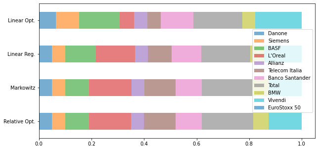
Although, strictly speaking, the linear-optimization tracking portfolio cannot fairly be compared with those of the preceding approaches, the results in the end do not differ greatly. The tracking portfolios’ structures are, within certain limits, quite similar, so their quality measures in the validation period do not diverge dramatically either. The reason for this perhaps surprising similarity is not hard to see. The two preceding approaches (the Markowitz approach and regression subject to constraints) essentially minimize the squared error (active return) between the tracking-portfolio and benchmark returns, whereas linear optimization minimizes the sum of the absolute values of the negative errors. If, in the estimation period, the observed return errors are distributed roughly symmetrically around zero and there are no serious outliers, then—apart from the squaring of the error terms—the linear-optimization objective is only scaled somewhat differently from that of the first two approaches, which has little effect on the location of the optimum. In that case, all three approaches yield quite similar tracking-portfolio structures.
Code
from matplotlib.pyplot import *
fig, ax = subplots()
df = pd.DataFrame({'Relative Opt.' :[round(x,4) for x in res1.x],
             'Markowitz' : [round(x,4) for x in res2.x],
              'Linear Reg.' : [round(x,4) for x in res3.x],
              'Linear Opt.' : [round(x,4) for x in res4.x[:11]]},
          index=ex_returns.columns).T
df.plot(kind='bar',stacked=True, ax=ax, figsize=(10,5))
ax.legend(loc=10);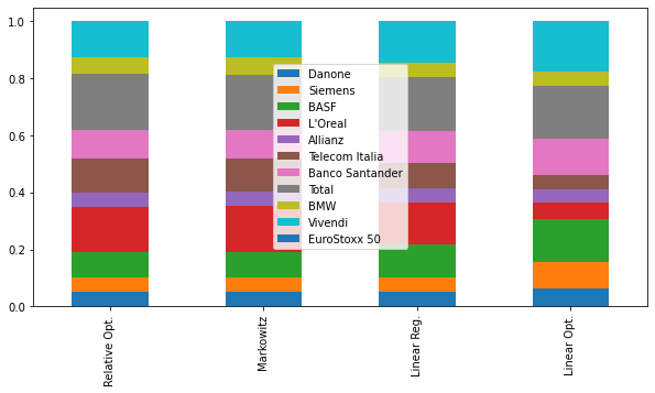
8.5 Summary
In this chapter you have learned the key concepts and goals of index tracking and clearly distinguished them from active portfolio strategies. You can compute and interpret the tracking error—the central metric—to assess how well an index-replication strategy performs. You can also compare the various index-tracking approaches and analyze their strengths and weaknesses on a sound basis. You have learned to formulate an index-tracking problem as an optimization task and to give an economic interpretation of the resulting portfolio weights. With this foundation, you can implement an index-tracking strategy in Python and critically assess its replication accuracy, stability, and practical usability.
8.6 Further reading and references
- finanzfluss/Maximilian Thomaser (2025). ETF replication methods compared.
- Poddig, T., Brinkmann, U., Seiler, K. (2009). Portfolio Management: Konzepte und Strategien, 2. Auflage, Uhlenbruch Verlag, Wiesbaden.
- Portfolio Optimizer (2023). Index Tracking: Reproducing the Performance of a Financial Market Index (and more).
Go deeper
Experience this chapter in the live seminar
In the in-house seminar Quant Portfolio Management, you will work through these methods hands-on in Python — with personal feedback, tailored case studies, and direct exchange with Prof. Dr. Thomas Mählmann.
Learn more about the seminar →