5  The Black-Litterman Model

Source

5.1 Learning Objectives

After completing this chapter, you will be able to …

• explain the basic idea and objective of the Black-Litterman model, in particular in comparison with the classical mean-variance optimization according to Markowitz.

• explain the individual components of the Black-Litterman model, including market equilibrium returns, subjective market expectations (views) as well as their uncertainties.

• formally formulate your own market expectations and integrate them consistently into a portfolio optimization model using the Black-Litterman approach.

• implement and interpret the calculation of posterior expected returns with the Black-Litterman model in Python.

• critically analyze the effects of different view weightings and confidence levels on portfolio allocations and use them for practical investment decisions.

5.2 Introduction and motivation: Deficiencies of portfolio optimization according to Markowitz

Markowitz’s portfolio selection theory, presented in the chapter “Absolute Portfolio Optimization”, is a widely accepted quantitative method for describing the trade-off between the two basic objectives of an investment: maximizing return and minimizing risk. It still forms the academic framework of portfolio theory. In practice, however, the Markowitz approach has gained only limited acceptance, owing to several serious problems. The four main problems in applying the classical approach are (cf. Drobetz, 2002, p. 4 ff.):

• Extreme portfolio allocations

  Optimized portfolios frequently contain extreme weights on both the long and the short side. Such weights could not be implemented in practice, if only for institutional and legal reasons. Mean-variance optimization tends toward extreme weights even under restrictions, such as a ban on short sales.

• Sensitivity of the portfolio weights

  Another problem is the strong sensitivity of the portfolio weights to changes in the inputs. Changes in the expected returns in particular lead to unrealistically large rebalancing within the portfolio. This causes high transaction costs, and an excessively high rebalancing frequency also makes portfolio management inconsistent and hard to communicate.

• Information aggregation

  The Markowitz approach requires specifying the expected returns of all securities together with the associated variance-covariance matrix. The difficulty of producing high-quality return forecasts, and the fact that portfolio managers usually have reliable expected returns only for selected classes of securities, makes assembling the input matrices for mean-variance optimization a major challenge.

• No possibility of making statements about forecast quality

  Using various analytical tools, portfolio managers often have differing levels of confidence in their forecasts. The Markowitz approach cannot take such differences in forecast quality into account.

These problems, which arise when classical portfolio theory is applied in practice, mean that the model can be implemented only to a limited extent. Trying to make it more realistic through various restrictions often takes disproportionate effort. This was what prompted Black and Litterman to develop a portfolio-management model that better addresses the deficiencies of the classical approach discussed above.

5.3 The approach of the Black-Litterman method

This section describes the basic procedure of the Black-Litterman method, which the following sections then formalize. The account here draws on the original source, Black and Litterman (1992); a very illustrative presentation of the method’s practical implementation can be found in Idzorek (2004).

The Black-Litterman method is always anchored to a reference portfolio that the portfolio manager specifies a priori. This portfolio should reflect the investor’s long-term investment behavior. If the manager has no views of their own about the future returns of the securities in the portfolio, they implicitly accept the implied expected returns (derived from the reference-portfolio weights), and the security weights then coincide with those of the reference portfolio. The method allows any number of return forecasts to be incorporated into the optimization while accounting for forecast quality. Both absolute forecasts about a security’s expected return level and relative forecasts about stronger- and weaker-performing securities can be built in.

The result is a revised return vector that shifts from the implied returns toward the subjective expected returns. This revised vector can then be passed to a mean-variance optimization routine. The Black-Litterman method thus produces intuitive changes in the portfolio weights that are consistent with the subjective forecasts and therefore easier to implement in practice.

Note that Black-Litterman is not an alternative optimization technique. Rather, it is a flexible way of adjusting return forecasts toward one’s own expected returns, starting from a neutral reference portfolio.

5.4 Reference portfolios and implied returns as the starting point of the Black-Litterman method

The innovative Black-Litterman method (1992) aims to overcome the weaknesses of Markowitz optimization listed above and thus to create a model better suited for practical use. The model’s most important feature is that it can consistently combine implied returns — explained below — with subjective expectations about the price development of the securities in the portfolio.

The implied returns that form the starting point of the Black-Litterman method are obtained by reverse optimization. First, the portfolio manager determines the medium- to long-term weights of the securities in the portfolio. These reference weights can be the equilibrium weights (based on relative market capitalization) underlying the CAPM, or they can result from the manager’s strategic considerations. Black and Litterman (1991, p. 3) suggest using the implied equilibrium returns derived from the market capitalizations as the starting point:

“Our model does not assume that the world is always at the CAPM equilibrium, but rather that when expected returns move away from their equilibrium values, imbalances in markets will tend to push them back. Thus, we think it is reasonable to assume that expected returns are not likely to deviate too far from equilibrium values. This intuitive idea suggests that the investor may profit by combining his views about returns in different markets with the information contained in the equilibrium.”

In the Markowitz method, a utility-maximizing portfolio manager with utility function \(U(w)=\mu_P-\frac{\lambda}{2} \sigma^2_P\) maximizes utility by optimally allocating the budget across the securities in the portfolio, given a vector of expected returns \(\mu\) and a variance-covariance matrix \(\Sigma\) of the returns. Without restrictions, the maximization problem is:

\[ (1) \quad U(w) =w^{T}\mu-\frac{\lambda}{2}w^{T}\Sigma w \rightarrow \max_{w}! \]

with the solution

\[ (2) \quad w^*=(\lambda \Sigma)^{-1}\mu . \]

In the Black-Litterman method, however, \(w^*\) is known from the outset — either through the CAPM equilibrium (the market-capitalization weights) or through strategically chosen weights. Reverse optimization then determines the expected returns required to reproduce exactly these reference weights \(w_{REF}\) in the Markowitz method. These returns are called implied returns \(\Pi\) or, when the market portfolio is the reference portfolio, equilibrium returns. Reverse optimization is simply a rearrangement of formula (2):

\[ (3) \quad \Pi=\lambda \Sigma w_{REF} . \]

To account explicitly for the uncertainty about the future expected returns \(\mu\), these are treated as random quantities. Assuming that expected values have a lower variance than the underlying random variables themselves, the a-priori distribution of \(\mu\) in the Black-Litterman model can be written as

\[ (4) \quad \mu_{a-priori} \sim N(\Pi, \tau \Sigma) , \]

where \(N(.)\) denotes the normal distribution. As for dimensions, \(\mu\) and \(\Pi\) are \(N×1\) vectors and the variance-covariance matrix \(\Sigma\) is an \(N×N\) matrix, where \(N\) is the number of securities. The parameter \(\tau\) is the proportionality factor relating the historical return volatility to the volatility of the expected return. The greater the manager’s confidence in the reference portfolio, the smaller \(\tau\) should be. The implied (or equilibrium) returns \(\Pi\) thus serve as the a-priori estimator of the expected returns \(\mu\). Setting \(\tau=0\) would assume no uncertainty about the future expected returns, so that they equal the historical values.

The next step combines the a-priori distribution of \(\mu\) with the portfolio manager’s individual return forecasts to obtain the a-posteriori distribution.

5.5 Connecting the reference portfolio with return forecasts

5.5.1 Specification of return forecasts in the Black-Litterman model

The decisive step in formalizing the Black-Litterman method is specifying the subjective expected returns (forecasts, opinions, or “views”), which is again done as a probability distribution.

As a rule, portfolio managers hold expectations about the future returns of some of the securities in the portfolio that deviate from the implied returns. The Black-Litterman model can incorporate both absolute and relative return forecasts into the asset-allocation process, and it is not necessary to specify an expected return for every security in the portfolio.

The following examples illustrate how absolute (A) and relative (B and C) expected returns can be expressed in the Black-Litterman model.

• 1. “Security A will generate a return of 6% (approx. 1.5% below the implied return).”
• 2. “Security E will generate a return that is 5% higher than security C.”
• 3. “Securities B and D will outperform securities A and C by 10%.”

Once the investor has stated, in words, all expectations that deviate from the implied returns (as in the examples above), these must be put into a form that can be integrated into the Black-Litterman process.

The model assumes that the manager’s expectations (forecasts) can be expressed, via the following formula, as \(k\) different linear combinations of the \(N\) securities, where \(k\) is the number of forecasts made.

\[ (5) \quad P \cdot \mu = V + \epsilon . \]

The vector of return forecasts \(V\) has dimension \(k×1\), and \(\epsilon\) is the \(k×1\) vector of forecast errors. The matrix \(P\) assigns the return forecasts (opinions or “views”) \(V\) to the correct securities: each expectation is mapped to the securities by a \(1×N\) vector (a row of \(P\)), so \(P\) is in general a \(k×N\) matrix, and each row of \(P\) represents a so-called “view portfolio”. The first element of \(V\) gives the magnitude of the first return forecast, and the first element of \(\epsilon\) its associated estimation error.

The forecasts (views) are given an estimation error, since in practice they cannot be stated with certainty. The error vector \(\epsilon\) is assumed to be independent and normally distributed. Forecast quality is measured in the Black-Litterman method by \(\Omega\), the variance-covariance matrix of the forecast errors. Because the forecasts are assumed independent of one another, the \(k×k\) matrix \(\Omega\) reduces to a diagonal matrix carrying the variances of the estimation errors \(\epsilon\) along its diagonal. The forecasts are assumed to be normally distributed:

\[ (6) \quad P \cdot \mu \sim N(V, \Omega) . \]

In a seven-security example with the securities \({A,B,C,D,E,F,G}\), the above forecasts (A), (B) and (C) would be formalized as follows:

\[ (7) \quad P \cdot \left( \begin{array}{rrrr} \mu_A \\ \mu_B \\ \mu_C \\ \mu_D \\ \mu_E \\ \mu_F \\ \mu_G \\ \end{array}\right) = \left( \begin{array}{rrrr} 0.06 \\ 0.05 \\ 0.10 \\ \end{array}\right) + \left( \begin{array}{rrrr} \epsilon_{(A)} \\ \epsilon_{(B)} \\ \epsilon_{(C)} \\ \end{array}\right) \ \]

with

\[ (8) \quad P=\left( \begin{array}{rrrr} 1 & 0 & 0 & 0 & 0 & 0 & 0 \\ 0 & 0 & -1 & 0 & 1 & 0 & 0 \\ -0.49 & 0.45 & -0.51 & 0.55 & 0 & 0 & 0 \\ \end{array}\right) .\]

The first row of \(P\) represents the absolute expectation (A). Since A is the first security in the example portfolio and the expectation concerns only this security, the first entry of the first row equals one and all other entries of the first row of \(P\) are zero.

The second row represents the relative expectation (B). A weight-neutral portfolio is formed by putting the stronger stock in the long position (value: 1) and the weaker stock in the short position (value: –1). The size of the outperformance appears in the second entry of the vector \(V\) (value: 0.05).

The third row of \(P\) represents the most complex case — simultaneous relative expected returns for more than two securities — illustrated here by expectation (C). As in a type-(B) relative expectation, the values of the stronger-performing stocks must sum to one and those of the outperformed securities to minus one. Within each of the two groups, the value (one or minus one) is split in proportion to market capitalization (assumed arbitrarily here). The entries of the third row of \(P\) were computed from formula (9):

\[ (9) \quad P^T_{3.} = \left( \begin{array}{rrrr} \frac{MCap_A}{MCAP_{A+C}} \\ \frac{MCap_B}{MCAP_{B+D}} \\ \frac{MCap_C}{MCAP_{A+C}} \\ \frac{MCap_D}{MCAP_{B+D}} \\ 0 \\ 0 \\ 0 \\ \end{array}\right) = \left( \begin{array}{rrrr} -0.49 \\ 0.45 \\ -0.51 \\ 0.55 \\ 0 \\ 0 \\ 0 \\ \end{array}\right) , \]

with \[ MCap_i: \text{market capitalization of security i} . \]

If the manager does not know the degree of uncertainty (the variance) of their expectations ex ante, the variance of the forecast portfolios (view portfolios) can be used instead:

\[ (10) \quad \Omega_{kk}=P_{k.} \tau\Sigma \space P^T_{k.}.\]

Since the forecast quality is unknown in this example, the variance-covariance matrix of the estimation errors, \(\Omega\), is approximated using formula (10). With \(\tau=1\) this yields:

\[ (11) \quad \Omega=\left( \begin{array}{rrrr} 0.0065 & 0 & 0 \\ 0 & 0.0037 & 0 \\ 0 & 0 & 0.0016 \\ \end{array}\right). \]

5.5.2 The Black-Litterman formula

The Black-Litterman model assumes that the unknown a-posteriori distribution of the expected returns \(\mu\) is a mixture of the a-priori distribution — based on the implied (or equilibrium) returns \(\Pi\) — and the distribution of the return forecasts \(V\). The a-priori distribution of \(\mu\) is given in formula (4) and the distribution of the return forecasts in formula (6).

The optimal (a-posteriori) estimator of the vector of expected returns is the mean \(E(\mu_{a-posteriori})\) of the mixed (a-posteriori) distribution, which is computed as:

\[ (12) \quad E(\mu_{a-posteriori})=[(\tau\cdot\Sigma)^{-1}+P^T\Omega^{-1}P]^{-1}[(\tau\cdot\Sigma)^{-1}\Pi+P^T\Omega^{-1}V]. \]

The a-posteriori distribution of the expected returns is again normal:

\[ (13) \quad \mu_{a-posteriori} \sim N(E(\mu_{A-posteriori}), [(\tau\cdot\Sigma)^{-1}+P^T\Omega^{-1}P]^{-1}) . \]

Formula (12) is the foundation of the entire Black-Litterman method: it combines the implied returns and the subjective forecasts into a new, revised vector of expected returns. Passing this vector to a mean-variance optimization routine then yields the Black-Litterman portfolio weights.

5.6 Conclusion

Markowitz’s classical portfolio-theory approach is elegant and provides the framework of portfolio theory in the academic literature. As the examples in this course have shown, however, it can lead to considerable problems in practice. Because of these deficiencies, portfolio managers rarely use the traditional approach, or use it only in heavily modified form.

For this reason, Black and Litterman developed an innovative method in 1992 that lets portfolio managers start from stable equilibrium (implied) returns and incorporate subjective return forecasts — together with a degree of confidence in them — into the asset-allocation process. Ultimately, the Black-Litterman model computes a sophisticated weighted average of the implied returns and the subjective return forecasts.

The Black-Litterman method makes the portfolio weights far more realistic, since the managers’ expectations are clearly reflected and highly concentrated portfolios are avoided. For these reasons, the Black-Litterman model has established itself as a portfolio-management model at numerous financial firms since its publication in 1992.

5.7 Start of the case study

We begin by importing the required packages.

import pandas as pd
import numpy as np
from scipy.optimize import minimize
import matplotlib.pyplot as plt
import numpy.linalg as la

5.7.1 Loading and describing the data set

The data set contains price histories (start-of-month prices) for the following ten stocks: Alcoa, IBM, Intel, J.P. Morgan, Microsoft, AT&T, Cisco, Ebay, Costco, and Kraft Foods. The prices cover the period 12.2004-12.2009 (61 months).

# insert here your local directory path of the file 
# cd "..."

frame1 = pd.read_excel('Kapitel A3_3.xlsx', 'Tabelle1', index_col=0, parse_dates=True)

frame1.tail()

	AA	IBM	INTC	JPM	MSFT	T	CSCO	EBAY	COST	KFT
2009-08-03	12.05	118.05	20.32	43.46	24.65	26.05	21.60	22.14	50.98	28.35
2009-09-01	13.12	119.61	19.57	43.82	25.72	27.01	23.54	23.60	56.38	26.27
2009-10-01	12.42	120.61	19.11	41.77	27.73	25.67	22.81	22.27	56.85	27.52
2009-11-02	12.52	126.35	19.20	42.49	29.41	26.94	23.40	24.47	59.91	26.58
2009-12-01	16.30	132.57	20.59	41.53	30.96	28.32	24.18	23.80	60.05	27.49

From continuous (log) returns, we compute and annualize the historical means and the variance-covariance matrix of the returns.

# using log returns
returns = np.log1p(frame1.pct_change().dropna())

means = returns.mean().values*12 # annualised
Sigma = returns.cov().values*12 # annualised

The market capitalization of each stock was determined as of the cut-off date 01.09.2012. The relative market capitalizations of the ten stocks are stored in the array cap_weights, which at the same time represent the reference weights \(w_{REF}\).

# current market cap of stocks and calculation of cap weights
market_cap = pd.read_excel('Market Cap.xlsx', 'Tabelle1')
cap_weights = np.asarray(market_cap)/np.sum(np.asarray(market_cap))

5.7.2 Determination of the implied returns

Starting from the unrestricted Markowitz maximization problem, the reverse optimization presented above gives the implied returns that make the reference portfolio efficient: \(\Pi=\lambda\Sigma w_{REF}\). For the risk-aversion coefficient \(\lambda\), we choose the value 2.0 as an example.

# calculation of market cap implied expected returns; lambda=gamma
gamma = 2
implied = 2*(cap_weights.dot(Sigma))

As shown above, inserting the vector of implied returns for \(\mu\) reproduces the reference-portfolio weights as the optimization result.

\[ (2) \quad w_{REF}=(\lambda \Sigma)^{-1}\Pi. \]

# optimal weights implied by implied expected returns
# analytical solution w = inv(gamma * Sigma1)* implied
# analytical solution possible because of no constraints
# Of course, impl_weights must equal cap_weights
impl_weights = implied.dot(la.inv(gamma * Sigma))

# optimal Markowitz weights based on hist. returns
marko_weights = means.dot(la.inv(gamma * Sigma))

It must therefore hold that cap_weights=impl_weights. If \(\mu\) is estimated from the simple historical means (means), the classical Markowitz weights (marko_weights) result.

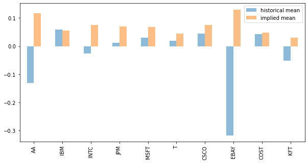
Let us now compare the historical means with the implied expected returns.

The bar chart compares the historical mean returns with the implied equilibrium returns based on the market-capitalization-weighted reference portfolio. Unlike the historical means, the implied expected returns are always positive and appear far more balanced and stable overall.

pd.DataFrame({'historical mean': means,'implied mean': implied[0,:]}, \
             index=frame1.columns).plot.bar(stacked=False, \
            alpha=0.5, figsize=(10,5));

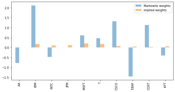
The following bar chart contrasts the (unrestricted) Markowitz weights based on historical returns with the reference weights based on the implied returns. The optimal portfolio based on the implied returns (which coincides with the reference portfolio) has entirely positive weights and hence no short positions. Unlike the portfolio optimized from historical mean returns, the equilibrium-return portfolio has no extreme weights at all, and it corresponds far more closely to common investment practice.

pd.DataFrame({'Markowitz weights': marko_weights,'implied weights': impl_weights[0,:]}, \
             index=frame1.columns).plot.bar(stacked=False, \
            alpha=0.5, figsize=(10,5));

5.7.3 Formulation and implementation of forecast opinions (views)

Having computed the implied returns, we now implement the portfolio manager’s subjective views. The implied returns serve as the starting point for the remaining calculations and, as a central “anchor”, stabilize the portfolio allocation. This anchoring role helps avoid the extreme allocations and high sensitivity that often arise in Markowitz optimization — one of the advantages of the Black-Litterman model over the mean-variance approach noted earlier. Since managers frequently hold a view on future returns that differs from the implied returns, their subjective assessments need to be incorporated.

Within the scope of the case study, the following security developments are assumed:

• View 1 For Ebay, portfolio management expects a return of 12.0% over the coming year.

• View 2 AT&T is assumed to earn a return 2.0% higher than Microsoft.

• View 3 The returns of Cisco and IBM will exceed those of Costco and Kraft Foods by 3.0%.

From the views specified by portfolio management, the vector \(V\) is:

\[ \quad V=\left( \begin{array}{rrrr} 12\% \\ 2\% \\ 3\% \\ \end{array}\right). \]

The relative and absolute views lead to the following forecast matrix \(P\):

\[ \quad P=\left( \begin{array}{rrrr} 0 & 0 & 0 & 0 & 0 & 0 & 0 & 1 & 0 & 0\\ 0 & 0 & 0 & 0 & -1 & 1 & 0 & 0 & 0 & 0\\ 0 & 0.69 & 0 & 0 & 0 & 0 & 0.31 & 0 & -0.36 & -0.64\\ \end{array}\right). \]

The absolute View 1 appears in the first row of the matrix. Row two represents View 2, a simple relative view, and View 3, a multiple relative view, is in row three of \(P\). The outperforming and underperforming securities (of the third view) enter the long and short portfolios, respectively, with their relative market-value weights.

# implementing the portfolio manager's view
P = np.zeros((3,10))
P[0,7]=1
P[1,4]=-1
P[1,5]=1
P[2,1]=0.69
P[2,6]=0.31
P[2,8]=-0.36
P[2,9]=-0.64

V = np.matrix([0.12, 0.02, 0.03])

Next we compute the Black-Litterman returns. But since each individual view is uncertain, we must first quantify each view’s estimation error. We do this by computing the diagonal matrix of estimation errors \(\Omega\) in proportion to the historical variance-covariance matrix, which gives the following \(\Omega\):

\[\Omega=\left( \begin{array}{rrrr} (P_1\Sigma P^T_1)\cdot \tau & 0 & 0 \\ 0 & \ddots & 0 \\ 0 & 0 & (P_k\Sigma P^T_k)\cdot \tau \\ \end{array}\right) = \left( \begin{array}{rrrr} 0.0526 & 0 & 0 \\ 0 & 0.0117 & 0 \\ 0 & 0 & 0.0064 \\ \end{array}\right). \]

For the proportionality factor \(\tau\) (the smaller it is, the greater the manager’s confidence in the reference portfolio), the literature recommends low values. Here we set \(\tau=0.2\).

Note: np.diag(np.diag(x)) first extracts the diagonal elements of the matrix \(x\) and then builds a diagonal matrix from them.

# calculation of omega: diagonal matrix containing variances of manager's
# forcasting errors

tau = 0.2
Omega = np.diag(np.diag((P.dot(tau*Sigma)).dot(P.T)))

We now blend the implemented views with the implied returns, following the central Black-Litterman equation (12) above:

\[ (12) \quad E(\mu_{a-posteriori})=[(\tau\cdot\Sigma)^{-1}+P^T\Omega^{-1}P]^{-1}[(\tau\cdot\Sigma)^{-1}\Pi+P^T\Omega^{-1}V]. \]

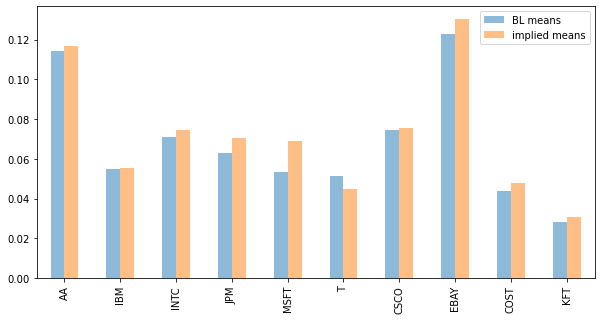
This yields the Black-Litterman returns. The bar chart below shows how far the views have moved them away from the implied returns.

# calculation of Black-Litterman expected returns
# imputs: tau, Omega, Sigma, P, implied, V

bl_means = la.inv(la.inv(tau*Sigma) + (P.T.dot(la.inv(Omega))).dot(P)).dot(\
    la.inv(tau*Sigma).dot(implied.T) + (P.T.dot(la.inv(Omega))).dot(V.T))

pd.DataFrame({'BL means': np.asarray(bl_means).T[0,:],'implied means': implied[0,:]}, \
             index=frame1.columns).plot.bar(stacked=False, \
            alpha=0.5, figsize=(10,5));

pd.DataFrame({'implied means': implied[0,:], 'BL means': np.asarray(bl_means).T[0,:],\
             'Difference (%)': np.round((np.asarray(bl_means).T[0,:]-implied[0,:]),4)*100}, \
             index=frame1.columns)

	implied means	BL means	Difference (%)
AA	0.117003	0.114132	-0.29
IBM	0.055150	0.054665	-0.05
INTC	0.074694	0.071138	-0.36
JPM	0.070246	0.063142	-0.71
MSFT	0.068769	0.053442	-1.53
T	0.044703	0.051446	0.67
CSCO	0.075445	0.074396	-0.10
EBAY	0.130241	0.122653	-0.76
COST	0.047745	0.044003	-0.37
KFT	0.030642	0.028216	-0.24

What is striking at first is that, in principle, the expected returns of all securities change, even though views were formulated for only some of them. This happens mainly because of the correlations between the individual returns, captured in the matrix \(\Sigma\).

The submitted view lowered the expected return for Ebay from about 13.0% to about 12.3%. The second view reduced the expected return for Microsoft by an absolute 1.53% and raised that for AT&T by an absolute 0.67%. This is intuitive: the return difference forecast by management (AT&T - Microsoft) was positive at 2.0%, whereas the difference in the implied returns is negative at -2.41% (4.47% - 6.88%). This worked against the Black-Litterman return of Microsoft and in favor of AT&T.

Assessing the effect of the multiple relative third view requires, unlike the first two views, looking at both the long (Cisco and IBM) and the short portfolio (Costco and Kraft Foods). Here the difference (+2.47%) between the weighted implied returns of the long (\(0.31\cdot7.54 +0.69\cdot5.52 = 6.15\)) and the short portfolio (\(0.36\cdot4.77+0.64\cdot3.06=3.68\)) is compared with the view (+3.0%). Again the direction of the change is intuitive: since the expected return difference between the long and short portfolios is smaller than the view, the difference is expected to widen. The return expectations therefore change so as to increase the gap between the long and short portfolios. In practice, the expected return of the long portfolio stays almost unchanged (IBM falls by an absolute 0.05%, Cisco by an absolute 0.1%), while the expected return of the short portfolio drops clearly: the Black-Litterman return for Costco is lower by an absolute 0.37% (relative: 7.75%), and Kraft Foods falls by a similar amount (relative: 7.84%). As noted at the outset, the return expectations change across all securities: those of Alcoa, Intel, and J.P. Morgan, which no view addressed, each fall by an absolute 0.29%, 0.36%, and 0.71%, respectively.

In short, every view for one security implicitly contains a forecast for every other security. This effect arises mainly from the multiplication of the matrices \(P\), \(\tau\Omega\), and \(\Sigma\) in the Black-Litterman formula (12).

5.7.4 Portfolio optimization according to Black-Litterman

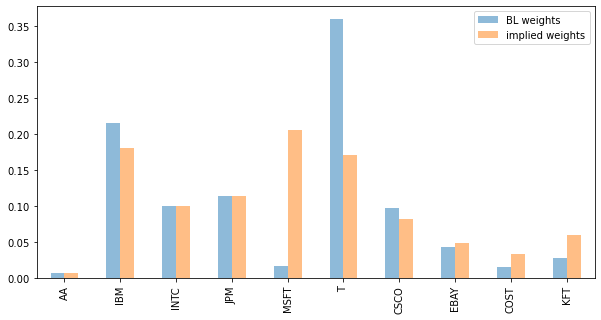
Optimizing the portfolio on the basis of the implied returns or the Black-Litterman returns determined above gives the following allocation.

# calculation of optimal portfolio weights using BL returns 
# and analytic formula
bl_weights = la.inv(gamma * Sigma).dot(bl_means)

pd.DataFrame({'BL weights': np.asarray(bl_weights)[:,0],'implied weights': impl_weights[0,:]}, \
             index=frame1.columns).plot.bar(stacked=False, \
            alpha=0.5, figsize=(10,5));

pd.DataFrame({'implied weights': impl_weights[0,:], 'BL weights': np.asarray(bl_weights)[:,0], \
              'Difference (%)': np.round((np.asarray(bl_weights)[:,0]-impl_weights[0,:]), 3)*100}, \
             index=frame1.columns)

	implied weights	BL weights	Difference (%)
AA	0.007369	0.007369	0.0
IBM	0.180836	0.214646	3.4
INTC	0.099716	0.099716	-0.0
JPM	0.113287	0.113287	0.0
MSFT	0.205001	0.016633	-18.8
T	0.170562	0.358930	18.8
CSCO	0.081912	0.097102	1.5
EBAY	0.048570	0.043521	-0.5
COST	0.033295	0.015655	-1.8
KFT	0.059452	0.028093	-3.1

As expected, only the weights of the securities addressed in the views changed. Alcoa, Intel, and J.P. Morgan, for which no subjective return estimates were submitted, enter the allocation unchanged, at the level of their relative market capitalizations in the initial portfolio. For IBM, Microsoft, AT&T, Cisco, Ebay, Costco, and Kraft Foods, for which forecasts were submitted, there are visible deviations. Microsoft’s share falls from 20.5% in the reference portfolio to 1.66%, a drop of an absolute 18.8%, while AT&T’s rises by an absolute 18.8% to 35.89% in the BL portfolio. The pattern is even clearer for the multiple relative view (View 3): here too, the long portfolio (IBM + Cisco) at an absolute +4.9% (= 3.4% + 1.5%) and the short portfolio (Costco + Kraft Foods) at an absolute -4.9% (= -1.8% - 3.1%) offset each other.

5.7.5 Portfolio optimization according to Black-Litterman and Markowitz in comparison

The following bar chart compares the allocation of the Black-Litterman portfolio with that of the Markowitz portfolio.

pd.DataFrame({'BL weights': np.asarray(bl_weights)[:,0],'Markowitz weights': marko_weights}, \
             index=frame1.columns).plot.bar(stacked=False, \
            alpha=0.5, figsize=(10,5));

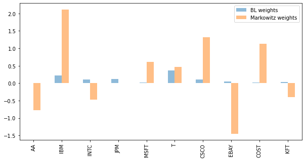
The first striking point is that the Black-Litterman weights are far more balanced than the composition of the Markowitz portfolio — the advantage of the Black-Litterman approach over Markowitz optimization noted earlier. The Black-Litterman portfolio aligns its allocation with the diversification intended by the portfolio manager (in line with the reference portfolio). It thereby meets the demands of practice: a sufficiently diversified portfolio, no extreme weights or short positions, and (where desired) alignment with a benchmark.

5.7.5.1 Markowitz portfolio optimization with restrictions: Corner portfolios

The Markowitz allocation shown above is often not realizable in practice — unlike the Black-Litterman allocation. For a Markowitz optimization, introducing constraints is one possible remedy: one could set individual upper and lower limits for securities, or, for company-policy reasons or external restrictions, impose a long-only constraint.

We therefore introduce a short-sale restriction below. In the case study, this long-only constraint affects only the Markowitz allocation, since the Black-Litterman weights are positive anyway. As noted earlier among the weaknesses of the Markowitz approach, however, a short-sale restriction frequently produces so-called corner portfolios — a problem that is clearly visible in the case study, too.

First we compute the efficient frontiers using the Black-Litterman expected returns and the classical, historically estimated expected returns.

5.7.5.2 Calculation of the efficient frontiers for BL and historically estimated expected returns

# use equal weights "Weight_1N" as starting values 
Weight_1N = np.tile(1.0/means.shape[0], means.shape[0])

We define the two target functions for the Global Minimum Variance Portfolio (GMVP) and the Maximum Return Portfolio (MRP).

# definition of target function for GMVP to be minimized
def calculate_portfolio_var(w,Sigma):
    # function that calculates portfolio risk
    w = np.matrix(w) # w is a row (not column!) vector
    return (w*Sigma*w.T)[0,0]

# definition of target function for MRP to be maximized
def calculate_negative_portfolio_ret(w,means):
    # function that calculates portfolio risk
    w = np.matrix(w) # w is a row (not column!) vector
    means = np.matrix(means)
    return -(w*means.T)[0,0]

# calculation of GMVP and MRP portfolio weights
# GMVP without short-sales
bnd=[(0, 1),(0, 1),(0, 1),(0, 1),(0, 1),
     (0, 1),(0, 1),(0, 1),(0, 1),(0, 1)] # only positive weights
cons = ({'type': 'eq', 'fun': lambda x:  np.sum(x)-1.0})

res2= minimize(calculate_portfolio_var, Weight_1N, args=Sigma, 
               bounds = bnd, method='SLSQP',constraints=cons,tol=1e-10, 
               options={'disp': True})
Weight_GMV = res2.x

# MRP portfolio
# for historic mean returns
res4= minimize(calculate_negative_portfolio_ret, Weight_1N, args=means, 
               bounds = bnd, method='SLSQP',constraints=cons,tol=1e-10, 
               options={'disp': True})
Weight_MRP_hist = res4.x

# for BL mean returns
res4= minimize(calculate_negative_portfolio_ret, Weight_1N, args=bl_means.T, 
               bounds = bnd, method='SLSQP',constraints=cons,tol=1e-10, 
               options={'disp': True})
Weight_MRP_bl = res4.x

Optimization terminated successfully    (Exit mode 0)
            Current function value: 0.01798288803981981
            Iterations: 20
            Function evaluations: 220
            Gradient evaluations: 20
Optimization terminated successfully    (Exit mode 0)
            Current function value: -0.059248481306705396
            Iterations: 13
            Function evaluations: 143
            Gradient evaluations: 13
Optimization terminated successfully    (Exit mode 0)
            Current function value: -0.12265320544211984
            Iterations: 10
            Function evaluations: 110
            Gradient evaluations: 10

# calculation of min and max target return
def calculate_portfolio_ret(w,means):
    # function that calculates portfolio risk
    w = np.matrix(w) # w is a row (not column!) vector
    means = np.matrix(means)
    return (w*means.T)[0,0]


# historic
min_hist = calculate_portfolio_ret(Weight_GMV, means)
max_hist = calculate_portfolio_ret(Weight_MRP_hist, means)

# BL
min_bl = calculate_portfolio_ret(Weight_GMV, bl_means.T)
max_bl = calculate_portfolio_ret(Weight_MRP_bl, bl_means.T)

We compute the efficient frontiers (the code is analogous to that in earlier chapters).

# efficient frontier with hist. mean returns
V_Target_hist = np.linspace(min_hist, max_hist, num=45)
V_Risk_hist = np.zeros(V_Target_hist.shape)
V_Return_hist = np.zeros(V_Target_hist.shape)
V_Weight_hist = np.zeros((V_Target_hist.shape[0], means.shape[0]))
for idx, Target_Return in enumerate(V_Target_hist):
    cons = ({'type': 'eq', 'fun': lambda x:  np.sum(x)-1.0},
            {'type': 'eq', 'fun': lambda x:  calculate_portfolio_ret(x,means)-Target_Return})
    res= minimize(calculate_portfolio_var, Weight_1N, args=Sigma, 
               bounds = bnd, method='SLSQP',constraints=cons,tol=1e-10)
    V_Weight_hist[idx, :] = res.x.T
    V_Return_hist[idx] = calculate_portfolio_ret(res.x,means)
    V_Risk_hist[idx] = np.sqrt(calculate_portfolio_var(res.x, Sigma))

# efficient frontier with hist. mean returns
V_Target_bl = np.linspace(min_bl, max_bl, num=45)
V_Risk_bl = np.zeros(V_Target_bl.shape)
V_Return_bl = np.zeros(V_Target_bl.shape)
V_Weight_bl = np.zeros((V_Target_bl.shape[0], means.shape[0]))
for idx, Target_Return in enumerate(V_Target_bl):
    cons = ({'type': 'eq', 'fun': lambda x:  np.sum(x)-1.0},
            {'type': 'eq', 'fun': lambda x:  calculate_portfolio_ret(x,bl_means.T)-Target_Return})
    res= minimize(calculate_portfolio_var, Weight_1N, args=Sigma, 
               bounds = bnd, method='SLSQP',constraints=cons,tol=1e-10)
    V_Weight_bl[idx, :] = res.x.T
    V_Return_bl[idx] = calculate_portfolio_ret(res.x,bl_means.T)
    V_Risk_bl[idx] = np.sqrt(calculate_portfolio_var(res.x, Sigma))

Plot of the curves (the code is analogous to that in earlier chapters).

fig1 = plt.figure(num=1, facecolor='w', figsize=(10, 5))
ax = fig1.add_subplot(111)
plt.plot(V_Risk_hist, V_Target_hist, 'g:', label='Hist.-Efficient frontier without short selling')
plt.plot(V_Risk_bl, V_Target_bl, 'g-', label='BL-Efficient frontier without short selling')
plt.plot(np.sqrt(np.diagonal(Sigma)), means, 'rx', label='Asset')
for i, txt in enumerate(frame1.columns):
   ax.annotate(txt, (np.sqrt(np.diagonal(Sigma))[i],means[i]))
plt.legend(loc='best',  frameon=True)
plt.xlabel('Standard deviation')
plt.ylabel('Expected return')
plt.show()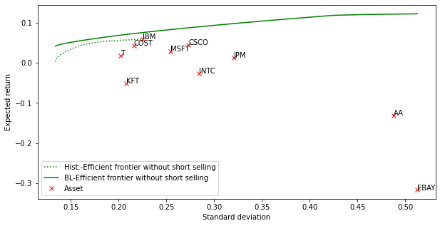

The efficient frontier of the Markowitz portfolios is considerably steeper than that of the Black-Litterman portfolios. The Black-Litterman portfolios are more broadly diversified and, in this case study, dominate the Markowitz portfolios at every point, always delivering a better return-risk ratio.

The following figure shows how the weights of the poorly diversified corner portfolios (along the efficient frontier) are composed in the Markowitz optimization with the long-only constraint (i.e., positive holding limits).

The optimal portfolios contain at most five securities (with a very small share for Microsoft in each case), and beyond a target return of a little over 5% the portfolio in fact consists of IBM alone.

fig2 = plt.figure(num=2, facecolor='w', figsize=(10, 5))
plt.stackplot(V_Target_hist, V_Weight_hist.T*100)
plt.axis([min_hist, max_hist, 0.0, 100.0])
plt.legend(list(frame1.columns),
           loc='upper left', bbox_to_anchor=(1.0, 1.0), frameon=False)
plt.xlabel('Target expected return')
plt.ylabel('Allocation weight (%)')
plt.title('Markowitz Allocations')
plt.show()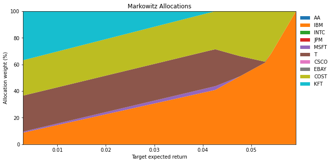

By contrast, the weights of the Black-Litterman portfolios along the efficient frontier behave far more evenly and form much more broadly diversified portfolios.

fig2 = plt.figure(num=2, facecolor='w', figsize=(10, 5))
plt.stackplot(V_Target_bl, V_Weight_bl.T*100)
plt.axis([min_bl, max_bl, 0.0, 100.0])
plt.legend(list(frame1.columns),
           loc='upper left', bbox_to_anchor=(1.0, 1.0), frameon=False)
plt.xlabel('Target expected return')
plt.ylabel('Allocation weight (%)')
plt.title('Black-Litterman Allocations')
plt.show()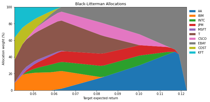

5.8 Summary

In this chapter you have met the basic idea and objective of the Black-Litterman model and understood its added value over classical mean-variance optimization. You can explain the model’s central components — market equilibrium returns, subjective market expectations, and their uncertainties. You are also able to formulate your own market expectations formally and integrate them consistently into a portfolio-optimization model. You have learned to implement and interpret the calculation of posterior expected returns with the Black-Litterman approach in Python. On this basis, you can critically analyze how different view weightings and confidence levels affect portfolio allocations and use them for practical investment decisions.

5.9 Further reading and references

• Black, F., Litterman, R. (1991). Global Asset Allocation with Equities, Bonds and Currencies. “Fixed Income Research”, Goldman, Sachs & Company, October.
• Black, F., Litterman, R. (1992). Global Portfolio Optimization. In: Financial Analysts Journal, September-October, pp. 28-43.
• Drobetz, W. (2002). Einsatz des Black-Litterman Verfahrens in der Asset Allocation. In: Dichtl, H., Kleeberg, J. M., Schlenger, C. (eds.). Handbuch Asset Allocation: Innovative Konzepte zur systematischen Portfolioplanung, pp. 204-239, Bad Soden: Uhlenbruch Verlag.
• Idzorek, T.M. (2004). A Step-by-Step Guide to the Black-Litterman Model, incorporating user-specified confidence levels. Working paper, Zephyr Associates, Inc.

Go deeper

Experience this chapter in the live seminar

In the in-house seminar Quant Portfolio Management, you will work through these methods hands-on in Python — with personal feedback, tailored case studies, and direct exchange with Prof. Dr. Thomas Mählmann.

Learn more about the seminar →