1  Foundations of classical (absolute) portfolio optimization

Source

1.1 Learning Objectives

After completing this chapter, you will be able to …

• explain the fundamental concepts of classical (absolute) portfolio optimization, in particular the relationship between expected return, risk (variance/standard deviation), and diversification.

• understand the mathematical foundations of Markowitz portfolio theory and correctly compute and interpret key quantities such as expected returns, variances, covariances, and correlation structures.

• formulate an optimization problem of classical portfolio optimization, including the target function (e.g., minimizing risk) and typical constraints (e.g., budget constraint, long-only constraint).

• derive the efficient frontier, plot it, and interpret it economically in order to identify risk-return-optimal portfolios.

• implement classical portfolio optimization in practice in Python, apply the relevant libraries, and critically analyze and contextualize the results.

1.2 Introduction

Portfolio construction (or portfolio implementation) is concerned with allocating the investment amount, by value, across the assets of the relevant investment universe.

When a portfolio is constructed by means of optimization, the optimal portfolio structure (the asset weights) is determined with respect to the particular objective pursued (operationalized through a target function TF), subject to any constraints.

1.3 \((\mu-\sigma)\)-efficient portfolios without a risk-free asset

What are optimal portfolios, and how can they be determined? To address this question, Markowitz (1952, 1959) narrows down the solution by excluding, from the set of all feasible and admissible portfolios, those that are clearly worse than others. The remaining so-called \((\mu-\sigma)\)-efficient portfolios are those that, for a given expected return \((\mu_{p})\), carry the minimum risk (variance or standard deviation of the return - \(\sigma^2_{p}\) or \(\sigma_{p}\)), or that, for a given level of risk, offer the maximum expected return. Such portfolios are said to dominate the others.

The selection of efficient portfolios rests, however, on two implicit assumptions:

• Investors prefer more return to less.
• If two portfolios have the same expected return, the one with the lower risk is chosen.

Markowitz thus implicitly assumes risk-averse investors. The dominance criterion can then be stated as follows:

An investment (portfolio) dominates another if it

• has a lower risk for the same return, or
• has a higher return for the same risk.

A portfolio is efficient precisely when no other portfolio exists that

• for the same expected return has a lower risk, or
• for the same risk has a higher expected return, or
• for a higher expected return simultaneously has a lower risk.

Using the dominance criterion, this yields the equivalent statement:

• A portfolio is efficient precisely when no other portfolio exists that dominates it.

The set of all efficient portfolios is also called the boundary (or curve) of efficient portfolios, or the efficient frontier.

1.4 Analytical determination of the efficient frontier

1.4.1 General case (including the long-only constraint)

To compute the efficient frontier, the following quadratic optimization problem (in matrix notation) must be solved:

\[ \begin{split} \\(OP1) \quad TF(w) = \sigma_P^2=w^{T}\Sigma w \rightarrow \min_{w}!, \\ \text{including the following conditions}\quad & \text{(a)}\ w^{T}\mu = \mu_{P}, \\ & \text{(b)}\ w^{T}\iota = 1 \quad \text{(budget constraint)}, \\ & \text{(c)}\ w\geqq 0 \quad \text{(long-only constraint)}, \end{split} \]

where

\[ w = \begin{bmatrix} w_1 \\ \vdots \\ w_N \end{bmatrix}, \quad \mu = \begin{bmatrix} \mu_1 \\ \vdots \\ \mu_N \end{bmatrix}, \quad \Sigma = \begin{bmatrix} \sigma_1^2 & \cdots & \sigma_{1N} \\ \vdots & \ddots & \vdots \\ \sigma_{N1} & \cdots & \sigma_N^2 \\ \end{bmatrix}. \]

• \(\mu_{P}\) : arbitrary, fixed prescribed portfolio return
• \(\mu\) : vector of expected asset returns
• \(\Sigma\) : future variance-covariance matrix of the asset returns
• \(\iota\) : unit vector (all elements of the vector are one)

Thus, for an arbitrary but fixed target portfolio return \(\mu_{P}\), the weights \(w_{i}\) (\(i=1, ..., N\), where \(N=\) the number of assets in the investment universe) are chosen so that the resulting portfolio risk (the variance of the portfolio return) is minimized. Solving problem OP1 yields one point \((\mu_{P}, \sigma^2_{p})\) on the efficiency curve. Repeating this for varying \(\mu_{P}\) then traces out the efficient frontier point by point.

1.4.2 Discussion of the constraints

Two constraints were introduced above: the budget constraint and the long-only constraint (short-selling prohibition). The budget constraint requires that the individual weights sum to one. The investor therefore cannot allocate more than the available capital across the assets, which rules out borrowing (leverage); at the same time, it forces full investment. If cash is to be taken into account, it is simply included in the investment universe as an asset with zero expected return and zero risk.

Short-selling is ruled out by requiring the individual weights to be non-negative. This restriction is common in practice and may stem, for example, from a legal or statutory ban on short-selling. A short sale is the sale of a security the seller does not own but has borrowed through securities lending. Anticipating falling prices, the short seller hopes to buy the security back later at a lower price, so that the gap between sale and repurchase price more than covers the lending fee.

Beyond these, a wide range of further constraints of a legal, statutory, or personal nature is possible. Examples include minimum and maximum holding limits for individual assets, maximum limits for groups of assets, a required minimum dividend yield for the portfolio, the exclusion of certain assets (e.g., “sin stocks”), adherence to sustainability criteria (e.g., a minimum portfolio ESG score), limits on turnover, transaction costs, and so on.

Clearly, adding (linear and nonlinear) constraints makes the optimization harder to solve. Since a problem may combine a highly nonlinear target function with equally complex, nonlinear constraints, one can intuitively expect that no solution method is both universally applicable and efficient at the same time.

1.4.3 Special case (without the long-only constraint)

1.4.3.1 Closed-form solution

As a rule, the optimization problem above has no closed-form solution. If, however, constraint (c) — the short-selling prohibition (the non-negativity condition) — is dropped, a Lagrangian approach yields the following closed-form solution for the optimal (i.e., variance-minimizing) portfolio weight vector \(w\) at a given expected portfolio return \(\mu_{P}\) (for the derivation see, e.g., Franzen and Schäfer, 2018, pp. 182-189)

\[ w = \frac{C\mu_P-A}{D}\Sigma^{-1}\mu + \frac{B-A\mu_P}{D}\Sigma^{-1}\iota, \]

where

\[ A =\mu^{T}\Sigma^{-1}\iota,\ B=\mu^{T}\Sigma^{-1}\mu,\ C =\iota^{T}\Sigma^{-1}\iota,\ D = B C - A^2. \]

The relationship between the given portfolio return \(\mu_P\) and the associated minimum portfolio risk \(\sigma_P\) can then be written as:

\[ \sigma_P = \sqrt{\frac{C\mu_P^2 - 2A\mu_P + B}{D}} = \sqrt{\frac{C}{D}\left(\mu_P-\frac{A}{C}\right)^2+\frac1{C}}, \]

and for the \((\mu_P-\sigma_{P})\) efficient frontier we have

\[ (1) \quad \mu_P = \begin{cases} \displaystyle \frac{A + \sqrt{D(C\sigma_P^2 - 1)}}{C}, & \mu_P > \frac{A}{C}; \\ & \\ \displaystyle \frac{A - \sqrt{D(C\sigma_P^2 - 1)}}{C}, & \mu_P < \frac{A}{C}. \end{cases} \]

1.4.3.2 Two-Fund Theorem

In the \((\mu-\sigma)\) coordinate system, the variance-minimizing portfolios — those that minimize risk (the variance or standard deviation of the return) for a given expected return — form a parabola (the feasibility curve, or “envelope”). Its efficient upper branch is the efficient frontier. The lower branch (the “inefficient frontier”) contains inefficient portfolios that are dominated by those on the efficient branch (for a given \(\sigma_{p}\), each has a larger \(\mu_{p})\). The vertex of the parabola, which separates the efficient from the inefficient branch, is the so-called minimum-variance portfolio (see below).

We can now draw on two theorems, due to Black (1972) and Merton (1972) (see also Benninga, 2014, Chapter 9), to span the entire parabola using any two base portfolios that lie on it.

The first theorem states that the weights of any portfolio on the parabola can be written as:

\[ (2) \quad w(c)=\frac{\Sigma^{-1}(\mu-c \iota)}{\iota^T[\Sigma^{-1}(\mu-c\iota)]},\]

where \(c\) is an arbitrary constant and \(\iota\) is the unit vector of dimension \(N\). Varying \(c\) produces different points on the parabola. We now pick any two base portfolios \(X\) and \(Y\) on it — for example, \(c=2\) for \(X\) and \(c=4\) for \(Y\).

The second theorem states that, given two base portfolios \(X\) and \(Y\) on the parabola, any other portfolio \(Z\) (point on the parabola) can be written as a convex combination of \(X\) and \(Y\): \(Z=\alpha X+(1-\alpha)Y\), where \(\alpha\) is an arbitrary constant. The expected return and risk of \(Z\) then follow as:

\[(3a) \quad \mu_{Z} = \alpha \mu_{X} + (1-\alpha) \mu_{Y} \]

\[(3b) \quad \sigma_{Z}=\sqrt{\alpha^2 \sigma^2_{X} + (1-\alpha^2) \sigma^2_{Y}+ 2\alpha (1-\alpha)Cov(X,Y)} \]

Here \(Cov(X,Y)\) denotes the return covariance between the two base portfolios.

Determining the parabola of variance-minimizing portfolios (efficient + inefficient branch) via the Two-Fund Theorem thus involves the following steps:

1. Choose the base portfolios \(X\) and \(Y\) by fixing two arbitrary values of \(c\).
2. Determine the weights of \(X\) and \(Y\) from equation (2).
3. Compute the expected return, the return variance, and the return covariance between \(X\) and \(Y\).
4. For many different values of \(\alpha\), compute the expected return and the return variance of \(Z\) from equations (3a) and (3b).

1.5 Two extreme optimal portfolios: MVP and MRP

The efficient frontier of optimal — i.e., \((\mu-\sigma)\)-efficient — portfolios is bounded by two extreme points: the minimum-variance portfolio (MVP) and the maximum-return portfolio (MRP).

The MVP is the portfolio with the globally lowest expected risk. Its optimization problem (in matrix notation) reads: \[ \begin{split} \\(OP2) \quad TF(w) = \sigma_P^2=w^{T}\Sigma w \rightarrow \min_{w}!, \\ \text{including the following conditions}\quad & \text{(a)}\ w^{T}\iota = 1 \quad \text{(budget constraint)}, \\ & \text{(b)}\ w\geqq 0 \quad \text{(long-only constraint)}, \end{split} \]

For the MRP, which lies at the other end of the efficient frontier, we have:

\[ (OP3) \quad TF(w) = \mu_{P}=w^{T}\mu \rightarrow \max_{w}! \]

The same constraints apply here. The MRP solution is therefore the portfolio invested 100% in the asset with the highest expected return.

1.6 Introduction of a risk-free asset

The problem of determining all efficient portfolios can be simplified by invoking Tobin separation, which reduces the task to determining a single efficient portfolio. Introducing a risk-free investment opportunity with interest rate \(r_{f}\) changes the problem: the investor can now form mixed portfolios from the risk-free asset and any portfolio on the efficient frontier — say portfolio P. For varying mixing ratios of \(r_{f}\) and P, the resulting \((\mu-\sigma)\) combinations lie on a straight line. The aim is to pair \(r_{f}\) with the particular portfolio TP on the efficient frontier whose mixed portfolios are not dominated by combinations of \(r_{f}\) with any other efficient portfolio P.

The portfolio TP is determined in the following way:

\[ \begin{split} \\(OP4) \quad TF(w) = \frac{\mu_p-r_f}{\sigma_p} \rightarrow \max_{w}!, \\ \text{including the following conditions}\quad & \text{(a)}\ w^{T}\iota = 1 \quad \text{(budget constraint)}, \\ & \text{(b)}\ w\geqq 0 \quad \text{(long-only constraint)}, \end{split} \]

Optimization problem OP4 amounts to maximizing the slope of the straight line running through the point \(r_{f}\) and through a point given by an efficient portfolio. This is equivalent to finding the tangent to the efficient frontier from the point \(r_{f}\). The expression \(\frac{\mu_p-r_f}{\sigma_p}\) is also known as the Sharpe ratio of portfolio \(P\).

The new efficient line available to the risk-averse investor consists of all combinations of the tangency portfolio TP and the risk-free investment \(r_{f}\). For this mixed portfolio, the expected return and risk are given by:

\[ \begin{split} \ \mu_{mix}=\alpha\mu_{TP}+(1-\alpha)r_{f} \ \text{and}\ \ \sigma_{mix}=\alpha \sigma_{TP}, \ \end{split} \]

where \(\alpha=\) the fraction of the investment amount allocated to the risky portfolio TP.

1.7 Determination of the investor-specific optimal portfolio

Determining the efficient portfolios, however, is not the end of the story. Ultimately, what we want is the portfolio that is optimal for the individual investor (Poddig et al., p. 84).

Within the framework of absolute optimization, we will not go into the determination of investor-specific optimal portfolios here. In the case study that follows, we focus solely on determining the complete efficient frontier; for investor-specific optimal portfolios, please refer to the subsequent chapters.

1.8 Start of the case study

We begin by importing the required packages.

import pandas as pd
import numpy as np
from scipy.optimize import minimize
import matplotlib.pyplot as plt
import numpy.linalg as la

1.8.1 Notes on implementing the numerical optimization in Python

In what follows, we carry out the numerical optimization of the respective target function (OP1-OP4) subject to its constraints using the minimize function from the scipy.optimize module. A few particularities are worth keeping in mind.

First, SciPy provides a “minimize” routine but no “maximize” function. Suppose we want to maximize the Sharpe ratio in optimization problem 4 (OP4). This looks like a problem at first, but it is easily resolved: maximizing the Sharpe ratio is the same as minimizing the negative Sharpe ratio — that is, simply the Sharpe ratio with a minus sign in front.

The basic procedure is always the same: first we write the target function to be optimized as a function, and then we define the structure of the constraints via the constraints object.

Let us walk through the individual entries to understand them better:

Since we use the SLSQP method in minimize (short for “Sequential Least Squares Programming”), the constraints object must be a tuple of Dictionaries containing the fields type and fun, together with the optional fields jac and args. We only need type, fun, and args. (A tuple is an immutable, fixed-length sequence of Python objects, written in round parentheses () with the elements separated by commas.)

The type is either eq or ineq, standing for equality and inequality, respectively. The fun is the function that defines the constraint — in our case, that the weights sum to one (the budget constraint). The way this has to be entered is a little cumbersome. eq means we are looking for a function whose output equals zero (that is what the equality refers to — equality to zero). The simplest way to achieve this is a Lambda function that returns the sum of the portfolio weights minus one; requiring its output to be zero is, by definition, the same as requiring the weights to sum to one.

Through the tuple bounds, which contains \(N\) identical bound=(minimum holding limit, maximum holding limit) tuples, we require every individual weight to lie between zero and one (the short-selling prohibition). The args are the arguments passed to the function being minimized (the target function) — all of its arguments EXCEPT the weight vector, which is of course the argument we vary to optimize the TF output.

Through the list initial weight we set the starting point for the numerical search for the optimal weights. The basic code for calling the minimize function therefore looks as follows:

# basic structure of code for optimization
constraints = ({'type': 'eq', 'fun': lambda x: np.sum(x) - 1})
bound = (0.0,1.0)
bounds = tuple(bound for i in range(number_of_assets))
minimize(target_function, initial_weights, args=args,
               method='SLSQP', bounds=bounds, constraints=constraints)

minimize returns the array x containing the optimized weights.

1.8.2 Loading and describing the data set

The example investment universe for the case study comprises ten companies from the following industries: technology, healthcare, food, pharmaceuticals, energy, and aerospace. The companies are: Abbott Laboratories (ABT), Boeing Industries (BA), Costco Wholesale (COST), Cisco Systems (CSCO), IBM (IBM), Intel (INTC), Merk (MRK), Microsoft (MSFT), AT&T (T), and Exxon Mobil Corporation (XOM).

The data set consists of beginning-of-month prices (“Adjusted Close”) over the 5-year period from 1.12.2004 to 1.12.2009, giving 61 time-series observations.

# insert here your local directory path of the file 'Kapitel A1.xlsx'
# cd "..."

frame = pd.read_excel('Kapitel A1.xlsx', 'Tabelle1', index_col=0, parse_dates=True)

frame.head()

	ABT	BA	COST	CSCO	IBM	INTC	MRK	MSFT	T	XOM
2004-12-01	46.65	51.77	48.41	19.32	98.58	23.39	32.14	26.72	25.77	51.26
2005-01-03	45.02	50.60	47.27	18.04	93.42	22.45	28.05	26.28	23.76	51.60
2005-02-01	45.99	54.97	46.59	17.42	92.58	23.99	31.70	25.16	24.06	63.31
2005-03-01	46.62	58.46	44.18	17.89	91.38	23.23	32.37	24.17	23.69	59.60
2005-04-01	49.16	59.52	40.63	17.27	76.38	23.52	33.90	25.30	23.80	57.03

1.8.3 Estimation of the input data for the optimization

All of the optimization problems above require two inputs: the vector of expected future asset returns \(\mu\) and the future variance-covariance matrix \(\Sigma\). Several methods are available for estimating these parameters.

The simplest conceivable approach uses the historical mean and empirical variance of an observed return series as estimators of the expected return and the future variance. Likewise, the empirical covariance of two return series serves as an estimator of their future covariance. This approach is known as simple history-based estimation. We use it here for forecasting returns and risk because it is easy to implement and intuitive, even though the results it produces are, as a rule, rather poor. Its use is justified solely by the didactic aim of demonstrating the various portfolio-optimization procedures from a methodological standpoint: these do require forecasts, but the quality of those forecasts is immaterial for the purpose at hand.

Poddig et al. (2009, pp. 116-121) give an overview of more sophisticated methods for forecasting returns and risk.

We first compute discrete monthly returns via frame.pct_change(), add one, and take the logarithm (via log1p) to obtain continuous (log) returns. We then apply the estimation to these and store the historically estimated (annualized) means and the empirical variance-covariance matrix in the arrays means and Sigma.

# simple, historical estimation based on log returns
log_returns = np.log1p(frame.pct_change().dropna()) 
means = log_returns.mean().values*100*12 # annualised
Sigma = log_returns.cov().values*12 # annualised

1.8.4 Application of absolute portfolio optimization

1.8.4.1 Computation of the minimum-variance portfolio (MVP)

1.8.4.1.1 Without the long-only constraint

We start by formulating the target function of optimization problem OP2 in the function calculate_portfolio_var. Via matrix(w) we turn the array w into a row vector of dimension \(1xN\).

# definition of target function to be minimized
def calculate_portfolio_var(w,Sigma):
    # function that calculates portfolio risk
    w = np.matrix(w) # w is a row (not column!) vector
    return (w*Sigma*w.T)[0,0]

As starting weights for the optimization we use an equally weighted portfolio. The call np.tile(A,x) generates an array that contains the value A x times. We obtain the number of assets in our example universe via means.shape[0].

# use equal weights "Weight_1N" as starting values 
Weight_1N = np.tile(1.0/means.shape[0], means.shape[0])

We are now ready to optimize; the optimized weights are stored in the array Weight_MV1. Setting options={'disp': True} displays general information about the optimization run, and tol controls the accuracy of the solution.

# unconstrained portfolio (only sum(w) = 1 )
cons = ({'type': 'eq', 'fun': lambda x:  np.sum(x)-1.0})
res1= minimize(calculate_portfolio_var, Weight_1N, args=Sigma,
              method='SLSQP',constraints=cons, tol=1e-10,
              options={'disp': True})
Weight_MV1 = res1.x

Optimization terminated successfully    (Exit mode 0)
            Current function value: 0.010828658442158556
            Iterations: 31
            Function evaluations: 341
            Gradient evaluations: 31

For better readability, we convert Weight_MV1 into a DataFrame.

pd.DataFrame([round(x,4) for x in Weight_MV1],index=frame.columns).T

	ABT	BA	COST	CSCO	IBM	INTC	MRK	MSFT	T	XOM
0	0.4359	-0.0418	0.2083	-0.0125	0.141	0.0902	-0.1451	-0.0239	0.0445	0.3035

Positive weights represent long positions and negative weights short positions; assets with negative weights are therefore sold short.

1.8.4.1.2 The Long-only constraint

We now impose the restriction to non-negative weights via a list of ten (0, 1) tuples.

# positive weight portfolio
bnd=[(0, 1),(0, 1),(0, 1),(0, 1),(0, 1),
     (0, 1),(0, 1),(0, 1),(0, 1),(0, 1)] # only positive weights
cons = ({'type': 'eq', 'fun': lambda x:  np.sum(x)-1.0})

res2= minimize(calculate_portfolio_var, Weight_1N, args=Sigma, 
               bounds = bnd, method='SLSQP',constraints=cons,tol=1e-10, 
               options={'disp': True})
Weight_MV2 = res2.x

Optimization terminated successfully    (Exit mode 0)
            Current function value: 0.012112846573987465
            Iterations: 21
            Function evaluations: 231
            Gradient evaluations: 21

pd.DataFrame([round(x,4) for x in Weight_MV2],index=frame.columns).T

	ABT	BA	COST	CSCO	IBM	INTC	MRK	MSFT	T	XOM
0	0.3617	0.0	0.1652	0.0	0.1621	0.0137	0.0	0.0	0.0523	0.2449

A striking feature of this solution is that four of the ten stocks drop out of the optimized portfolio, and that more than 60% of the portfolio is concentrated in just two stocks, ABT and XOM. To obtain a more diversified portfolio, we add a further constraint when computing a third MVP: each asset must be held with a weight of at least 5% but no more than 35%.

1.8.4.1.3 Additional constraint: holding limits (min=5%, max=35%)

# position constraints
bnd=[(0.05, 0.35),(0.05, 0.35),(0.05, 0.35),(0.05, 0.35),(0.05, 0.35),
     (0.05, 0.35),(0.05, 0.35),(0.05, 0.35),(0.05, 0.35),(0.05, 0.35)]
cons = ({'type': 'eq', 'fun': lambda x:  np.sum(x)-1.0})

res3= minimize(calculate_portfolio_var, Weight_1N, args=Sigma, 
               bounds = bnd, method='SLSQP',constraints=cons,tol=1e-10, 
               options={'disp': True})
Weight_MV3 = res3.x

Optimization terminated successfully    (Exit mode 0)
            Current function value: 0.014612315837805704
            Iterations: 18
            Function evaluations: 198
            Gradient evaluations: 18

pd.DataFrame([round(x,4) for x in Weight_MV3],index=frame.columns).T

	ABT	BA	COST	CSCO	IBM	INTC	MRK	MSFT	T	XOM
0	0.3313	0.05	0.0689	0.05	0.1062	0.05	0.05	0.05	0.05	0.1935

1.8.4.2 Computation of the maximum-return portfolio (MRP) under the long-only constraint

We again start by formulating the target function of optimization problem OP3, in the function calculate_negative_portfolio_ret. Note: minimizing the expected portfolio return multiplied by -1 is equivalent to maximizing the return.

# definition of target function to be minimized
def calculate_negative_portfolio_ret(w,means):
    # function that calculates -1 times portfolio expected return
    w = np.matrix(w) # w is a row (not column!) vector
    means = np.matrix(means)
    return -(w*means.T)[0,0]

# positive weight portfolio
bnd=[(0, 1),(0, 1),(0, 1),(0, 1),(0, 1),
     (0, 1),(0, 1),(0, 1),(0, 1),(0, 1)] # only positive weights
cons = ({'type': 'eq', 'fun': lambda x:  np.sum(x)-1.0})

res4= minimize(calculate_negative_portfolio_ret, Weight_1N, args=means, 
               bounds = bnd, method='SLSQP',constraints=cons,tol=1e-10, 
               options={'disp': True})
Weight_MRP = res4.x

Optimization terminated successfully    (Exit mode 0)
            Current function value: -7.886975933686317
            Iterations: 2
            Function evaluations: 22
            Gradient evaluations: 2

pd.DataFrame([round(x,4) for x in Weight_MRP],index=frame.columns).T

	ABT	BA	COST	CSCO	IBM	INTC	MRK	MSFT	T	XOM
0	0.0	0.0	0.0	0.0	0.0	0.0	0.0	0.0	0.0	1.0

The portfolio is invested 100% in XOM, the stock with the highest mean return in the data set. To obtain a more broadly diversified portfolio, we could again add holding limits as a further constraint.

1.8.4.3 Computation of a point on the efficient frontier under the long-only constraint

We now determine a point on the efficient frontier by setting the target return \(\mu_P\) in optimization problem OP1 to, say, 6%. We implement this extra constraint in two steps. First we write the function calculate_portfolio_ret, which computes the expected portfolio return. Then we add it as a Lambda function to the tuple cons of constraint dictionaries.

# definition of function for portfolio expected return
def calculate_portfolio_ret(w,means):
    w = np.matrix(w) # w is a row (not column!) vector
    means = np.matrix(means)
    return (w*means.T)[0,0]

# positive weight portfolio
bnd=[(0, 1),(0, 1),(0, 1),(0, 1),(0, 1),
     (0, 1),(0, 1),(0, 1),(0, 1),(0, 1)] # only positive weights

cons = ({'type': 'eq', 'fun': lambda x:  np.sum(x)-1.0},
        {'type': 'eq', 'fun': lambda x:  calculate_portfolio_ret(x,means)-6.0})


res4= minimize(calculate_portfolio_var, Weight_1N, args=Sigma, 
               bounds = bnd, method='SLSQP',constraints=cons,tol=1e-10, 
               options={'disp': True})
Weight_tar6 = res4.x

Optimization terminated successfully    (Exit mode 0)
            Current function value: 0.0149725199855123
            Iterations: 13
            Function evaluations: 143
            Gradient evaluations: 13

Let us quickly verify that the optimized portfolio weights really do produce an expected portfolio return of 6%.

calculate_portfolio_ret(Weight_tar6,means)

6.000000000000562

pd.DataFrame([round(x,4) for x in Weight_tar6],index=frame.columns).T

	ABT	BA	COST	CSCO	IBM	INTC	MRK	MSFT	T	XOM
0	0.2001	0.0	0.149	0.0	0.1609	0.0	0.0	0.0	0.0	0.49

1.8.4.4 Computation of the complete efficient frontier under the long-only constraint

First we determine the range of expected returns spanned by the portfolios on the efficient frontier. This is the same as the range of target returns in optimization problem OP1, where the minimum target return equals the return of the MVP and the maximum target return equals the return of the MRP.

# calculation of min and max target return
# min: expected return of GMVP, max: expected return of MRP

min = calculate_portfolio_ret(Weight_MV2, means)
max = calculate_portfolio_ret(Weight_MRP, means)

Via np.linspace we now create the array V_Target with 45 evenly spaced target returns between the minimum and maximum defined above. We also define the arrays V_Risk and V_Return, in which we will later store the \(\sigma_P\) and \(\mu_P\) produced by the optimization, and the matrix V_Weight of dimension 45x10, whose rows hold the ten asset weights for each of the 45 optimized portfolios (one per target return).

We then loop over the array of target returns. We use enumerate to “carry along” the iteration index (here called idx), so that we can index the positions in the result arrays and in the weight matrix.

V_Target = np.linspace(min, max, num=45)
V_Risk = np.zeros(V_Target.shape)
V_Return = np.zeros(V_Target.shape)
V_Weight = np.zeros((V_Target.shape[0], means.shape[0]))
for idx, Target_Return in enumerate(V_Target):
    cons = ({'type': 'eq', 'fun': lambda x:  np.sum(x)-1.0},
            {'type': 'eq', 'fun': lambda x:  calculate_portfolio_ret(x,means)-Target_Return})
    res= minimize(calculate_portfolio_var, Weight_1N, args=Sigma, 
               bounds = bnd, method='SLSQP',constraints=cons,tol=1e-10)
    V_Weight[idx, :] = res.x.T
    V_Return[idx] = calculate_portfolio_ret(res.x,means)
    V_Risk[idx] = np.sqrt(calculate_portfolio_var(res.x, Sigma))

We now plot the resulting efficient frontier together with the positions of the ten assets.

fig1 = plt.figure(num=1, facecolor='w', figsize=(10, 5))
plt.plot(V_Risk, V_Target, 'g:', label='Efficient frontier without short selling')
plt.plot(np.sqrt(np.diagonal(Sigma)), means, 'rx', label='Asset')
plt.legend(loc='best',  frameon=False)
plt.xlabel('Standard deviation')
plt.ylabel('Expected return (%)')
plt.show()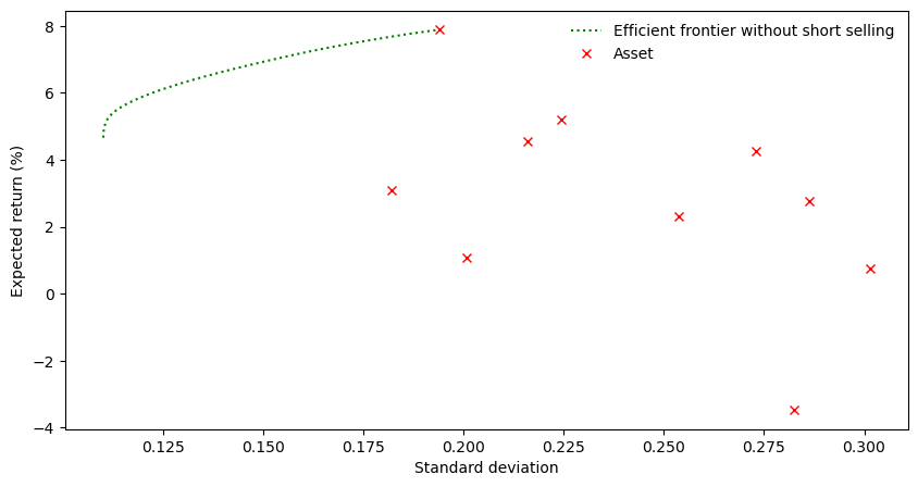

Next we plot the optimal weights across the 45 target returns.

fig2 = plt.figure(num=2, facecolor='w', figsize=(10, 5))
plt.stackplot(V_Target, V_Weight.T*100)
# colors=tuple([tuple(gray*np.ones(3)) for gray in np.linspace(0.4, 0.8, num=means.shape[0])]))
plt.axis([min, max, 0.0, 100.0])
plt.legend(list(frame.columns),
           loc='upper left', bbox_to_anchor=(1.0, 1.0), frameon=False)
plt.xlabel('Target expected return (%)')
plt.ylabel('Allocation weight (%)')
plt.show()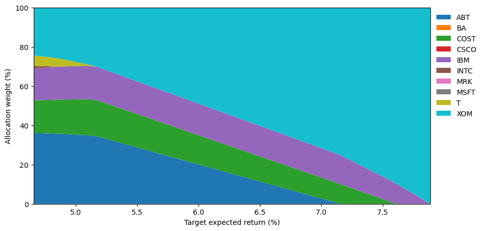

1.8.4.5 Computation of the complete efficient frontier under the long-only constraint

In the special case without the long-only constraint (i.e., with only the budget constraint), the parabola of variance-minimizing portfolios can also be obtained without numerical optimization, via a closed-form solution (see the discussion above). We now compute the parabola from equation (1). For this we need NumPy’s linear-algebra module numpy.linalg, which we imported above as la. Important: in the special case without the long-only constraint, the variance of the MVP satisfies \(\sigma^2_{MVP}=\frac{1}{C}\), where \(C=\iota^{T}\Sigma^{-1}\iota\) (for the derivation see, e.g., Franzen and Schäfer, 2018, p. 189).

inv is the function for computing a matrix inverse, and @ is the matrix-multiplication operator. Important: in Python, @ works as long as the length of a vector matches the length of the corresponding row/column of the matrix, so we do not need to apply the transpose operator T to means or iota.

First we create the unit vector of dimension \(N\) and extract the assets’ standard deviations.

iota = np.ones(means.shape)
Stdev = np.sqrt(np.diagonal(Sigma))

Next we compute the inverse of the variance-covariance matrix and the four quantities A, B, C, and D from equation (1).

inv_Sigma = la.inv(Sigma)
A = means @ inv_Sigma @ iota
B = means @ inv_Sigma @ means
C = iota @ inv_Sigma @ iota
D = B * C - A ** 2

We store the standard deviation of the MVP as sigma_gmv. This is the lower bound of the \(\sigma_P\) values for which we compute the two (efficient and inefficient) \(\mu_P\) values from equation (1). As the upper bound for the \(\sigma_P\) values we take the largest asset standard deviation (np.max(Stdev)). For 250 evenly spaced \(\sigma_P\) values within these bounds, we compute the efficient and inefficient branches of the parabola of variance-minimizing portfolios (in the arrays mu_p_efficient and mu_p_inefficient).

sigma_gmv = 1.0 / np.sqrt(C)
sigma_p = np.linspace(sigma_gmv, np.max(Stdev), num=250)
mu_p_efficient = (A + np.sqrt(np.abs(C * sigma_p ** 2 - 1.0) * D)) / C
mu_p_inefficient = (A - np.sqrt(np.abs(C * sigma_p ** 2 - 1.0) * D)) / C

Finally, we plot the efficient frontiers with and without the long-only constraint together in a single graph.

fig2 = plt.figure(num=1, facecolor='w', figsize=(10, 5))
plt.plot(sigma_p, mu_p_efficient, 'b-', label='Efficient frontier with short selling')
plt.plot(V_Risk, V_Target, 'g:', label='Efficient frontier without short selling')
plt.plot(np.sqrt(np.diagonal(Sigma)), means, 'rx', label='Asset')
plt.legend(loc='best',  frameon=False)
plt.xlabel('Standard deviation')
plt.ylabel('Expected return (%)')
plt.show()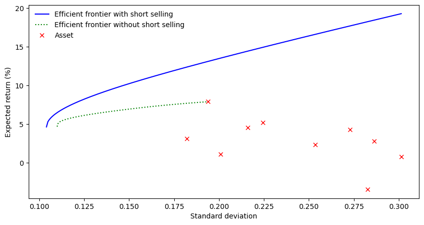

As expected, the efficient frontier without the long-only constraint lies above the one with it: each additional constraint narrows the space of feasible optimal portfolios further.

1.8.4.6 Computation of the efficient frontier based on the Two-Fund Theorem

Important: This approach is only valid if short selling is permitted!

In the first step we determine the weights (port1 and port2) of two base portfolios \(X\) and \(Y\) from equation (2) above. For the constant \(c\) we choose the values 2.0 and 4.0.

For both portfolios we compute the expected return and return variance, as well as the return covariance between \(X\) and \(Y\).

Note: the return covariance is given by \(Cov(X,Y)=w^{T}_X\Sigma w_Y\)

# use 2.0 and 4.0 as constant values
# calculate the two basis portfolios 1 and 2
port1 = (inv_Sigma*np.matrix(means-2.0).T)/np.sum(inv_Sigma*np.matrix(means-2.0).T)
port2 = (inv_Sigma*np.matrix(means-4.0).T)/np.sum(inv_Sigma*np.matrix(means-4.0).T)
covariance=(port1.T*Sigma*port2)[0,0]
ret1 = (np.matrix(means) * port1)[0,0] 
ret2 = (np.matrix(means) * port2)[0,0] 
var1 = (port1.T*Sigma*port1)[0,0]
var2 = (port2.T*Sigma*port2)[0,0]

Next, using formulas (3a) and (3b), we compute the expected return and return variance of a portfolio \(Z=\alpha X+(1-\alpha)Y\). Via np.linspace we pick 250 evenly spaced values of \(\alpha\) between 0 and 1.5, and store the resulting expected returns and risks of the 250 \(Z\) portfolios in the arrays Risk and Return. Again we use enumerate to index the arrays.

# construction of portfolios from the two basis portfolios for 
# different weights w
weight = np.linspace(0, 1.5, num=250)
Risk = np.zeros(weight.shape)
Return = np.zeros(weight.shape)
for idx, w in enumerate(weight):
    Return[idx] = w*ret1 + (1-w)*ret2
    Risk[idx] = np.sqrt(w**2 * var1 + (1-w)**2 * var2 + 2*w*(1-w)*covariance)
    

Finally, we plot the resulting efficient frontier together with the one computed numerically above for the case where short selling is not permitted.

fig3 = plt.figure(num=1, facecolor='w', figsize=(10, 5))
plt.plot(Risk, Return, 'b-', label='Efficient frontier with short selling')
plt.plot(V_Risk, V_Target, 'g:', label='Efficient frontier without short selling')
plt.plot(np.sqrt(np.diagonal(Sigma)), means, 'rx', label='Asset')
plt.legend(loc='best',  frameon=False)
plt.xlabel('Standard deviation')
plt.ylabel('Expected return (%)')
plt.show()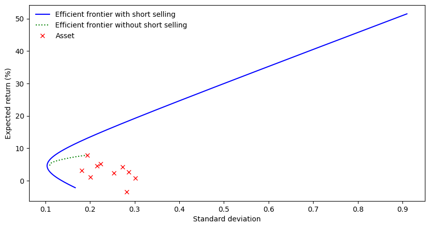

1.8.4.7 Determination of the tangency portfolio (TP) under the long-only constraint

As described above, the existence of a risk-free investment gives rise to a new efficient frontier. Determining the tangency portfolio TP (the portfolio with the maximum Sharpe ratio) comes down to one question: which portfolio maximizes the excess return (over the risk-free rate) per unit of portfolio risk?

We implement the target function of optimization problem OP4 in the function calc_neg_sharpe. It takes as inputs \(w\), \(\mu\), \(\Sigma\), \(r_f\), and the frequency freq of the return observations. For monthly returns, for instance, freq=12. To return the (negative) annualized Sharpe ratio, the expected portfolio return (portfolio_return) is multiplied by freq and the return standard deviation (portfolio_std) by the square root of freq. \(r_f\) should be given as an annual rate. Annualization is of course skipped (set freq to one) if the estimates of \(\mu\) and \(\Sigma\) are already annualized, as they are in our case.

Note that, in matrix notation, the portfolio variance is \(\sigma_P^2=w^{T}\Sigma w\). In the function we perform the matrix multiplication twice in succession via np.dot.

# definition of target function for maximum Sharpe portfolio
# "freq" denotes the return frequency (daily=252, monthly=12, annual=1, etc.)
def calc_neg_sharpe(weights, mean_returns, cov, rf, freq):
    portfolio_return = np.sum(mean_returns * weights) * freq
    portfolio_std = np.sqrt(np.dot(weights.T, np.dot(cov, weights))) * np.sqrt(freq)
    sharpe_ratio = (portfolio_return - rf) / portfolio_std
    return -sharpe_ratio

We put the complete optimization problem into the function max_sharpe_ratio. Two details are worth noting here:

1. We generate the tuple bounds, with identical position limits for all assets, neatly via a for loop.
2. We build the equally weighted starting portfolio as a list via num_assets*[1./num_assets,].

# function that implements the Sharpe portfolio optimization
def max_sharpe_ratio(mean_returns, cov, rf, freq):
    num_assets = len(mean_returns)
    args = (mean_returns, cov, rf, freq)
    constraints = ({'type': 'eq', 'fun': lambda x: np.sum(x) - 1})
    bound = (0.0,1.0)
    bounds = tuple(bound for asset in range(num_assets))
    result = minimize(calc_neg_sharpe, num_assets*[1./num_assets,], args=args,
                        method='SLSQP', bounds=bounds, constraints=constraints,tol=1e-10)
    return result

For an annual risk-free rate of 3%, we now compute the tangency-portfolio weights for our example investment universe.

# set annual risk-free rate to 3% and calculate maximum Sharpe portfolio
rf = 3.0
optimal_port_sharpe = max_sharpe_ratio(means, Sigma, rf, 1)

pd.DataFrame([round(x,4) for x in optimal_port_sharpe['x']],index=frame.columns).T

	ABT	BA	COST	CSCO	IBM	INTC	MRK	MSFT	T	XOM
0	0.0	0.0	0.0979	0.0	0.1474	0.0	0.0	0.0	0.0	0.7547

Evidently, the tangency portfolio is 75% XOM. A more broadly diversified portfolio would require maximum holding limits (e.g., 35%).

1.9 Summary

In this chapter you have met the fundamental concepts of classical portfolio optimization and seen how expected return, risk, and diversification relate to one another. You can follow the mathematical foundations of Markowitz portfolio theory and correctly compute and interpret key quantities such as expected returns, variances, covariances, and correlations. You are also able to formulate a classical portfolio-optimization problem with a suitable target function and typical constraints. You have learned to derive the efficient frontier, plot it, and interpret it economically. On this basis, you can implement classical portfolio optimization in Python and critically analyze and contextualize the results.

1.10 Further reading and references

• Benninga, S., (2014). Financial Modeling, 4th edition, MIT Press, London.
• Black, F. (1972). Capital Market Equilibrium with Restricted Borrowing. In: The Journal of Business Vol. 45, pp. 444-455.
• Franzen, D., Schäfer, K. (2018). Assetmanagement, 1. Auflage, Schäffer-Poeschel, Stuttgart.
• Markowitz, H. M. (1952). Portfolio selection. In: The Journal of Finance Vol. 7, pp. 77–91.
• Markowitz, H. M. (1959). Portfolio Selection: Efficient Diversification of Investments. John Wiley & Sons.
• Merton, R. C. (1972). An Analytic Derivation of the Efficient Portfolio Frontier. In: The Journal of Financial and Quantitative Analysis Vol. 7, pp. 1851-1872.
• Poddig, T., Brinkmann, U., Seiler, K. (2009). Portfolio Management: Konzepte und Strategien, 2. Auflage, Uhlenbruch Verlag, Wiesbaden.

Go deeper

Experience this chapter in the live seminar

In the in-house seminar Quant Portfolio Management, you will work through these methods hands-on in Python — with personal feedback, tailored case studies, and direct exchange with Prof. Dr. Thomas Mählmann.

Learn more about the seminar →