6  Accounting for Estimation Risk: Portfolio Resampling

Source

6.1 Learning Objectives

After completing this chapter, you will be able to …

• explain the concept of estimation risk in portfolio optimization and professionally assess its effects on the optimal portfolio weights.

• understand the principle of Michaud’s portfolio resampling, including the generation of simulated return and covariance estimates to reduce instabilities.

• implement resampling procedures in Python by performing repeated optimizations based on randomly drawn samples and aggregating the resulting portfolios.

• compare resampling-based portfolio weights with classical Markowitz portfolios and systematically evaluate differences in terms of stability, diversification, and robustness.

• apply portfolio resampling as a practice-oriented method for accounting for uncertainty in the input parameters in quantitative investment decisions, and critically reflect on it.

6.2 Introduction and motivation

The rationale for the resampling method rests on the recognition that any estimated efficient frontier is subject to uncertainty. The efficient frontier is derived from the input parameters (\(\mu\) and \(\Sigma\)). Since the true values of these parameters are unknown ex ante and can only be estimated, the true efficient frontier is itself unknown, and the frontier we obtain is merely an uncertain estimate of it. Uncertainty in the input parameters thus feeds directly into uncertainty in the estimated efficient frontier.

How can the uncertainty (the estimation risk) in the efficient frontier be quantified? And can this be used to build a new estimator that reduces the estimation risk — and thereby produces more stable portfolio weights that are less sensitive to changes in the input parameters \(\mu\) and \(\Sigma\)? The resampling method addresses these questions.

The method breaks down, in essence, into the following steps (see Michaud and Michaud, 2008, for more detail):

• First, estimate the input parameters \(\mu\) and \(\Sigma\), e.g. by simple historical estimation. We denote the set of estimated parameters by \(\theta\) and assume there are \(m\) securities.

• Next, determine the weights of the global minimum-variance portfolio (MVP) and the maximum-return portfolio (MRP). We denote the expected return of the MVP by \(L\) and that of the MRP by \(H\).

• We discretize the continuous efficient frontier by fixing the number \(K\) of target returns for which we compute it (the MVP for each target return). For example, if \(L=0.05\) and \(H=0.20\) and we choose \(K=16\) points, we compute the frontier for the target returns \(\{0.05; 0.06; ...; 0.19; 0.20\}\), giving \(16\) points on the efficient frontier.

• We then write the discretized efficient frontier as a matrix \(a_K\), each element of which is a portfolio weight. The matrix therefore has dimension \(Kxm\) (rows for the target returns, columns for the securities). The pair \((a_K, \theta)\) thus describes the efficient frontier obtained from the (e.g. historically) estimated parameters. In our example it has 16 rows (target returns, evenly spaced between \(L\) and \(H\)).

• We begin the Monte Carlo simulation by drawing a realization \(\theta_i\) from the probability distribution of \(\theta\); \(\theta_i\) and \(\theta\) are said to be “statistically equivalent”. This involves the following steps. Suppose our investment universe consists of \(m=5\) securities and our historical return time series has \(k=200\) observations. Using \(\theta\) (i.e. the historically estimated vector of expected returns \(\mu\) and the historical covariance matrix \(\Sigma\)), we assume a multivariate normal distribution for the return vector \(R_m\) of the \(m\) returns (i.e. \(R_m \sim N_m(\mu,\Sigma)\)) and, with a random number generator, draw five returns 200 times (i.e. one realization of \(R_m\)) from this assumed multivariate distribution (which need not be normal). From the simulated return time series we then compute the simulated \(\mu_i\) and \(\Sigma_i\), i.e. \(\theta_i\).

• Using \(\theta_i\), recompute the MVP (expected return \(L_i\)) and the MRP (expected return \(H_i\)), and split the interval \([L_i,H_i]\) into \(K\) evenly spaced target returns. Following the example above with \(K=16\), for \(L_i=0.03\) and \(H_i=0.25\) the target returns are \(\{0.030; 0.044; 0.058; ...; 0.236; 0.250\}\).

• Determine the efficient portfolio weights for each of the \(K\) points (the MVP weights for target returns of 0.030, 0.044, and so on). This yields a new \(K x m\) matrix \(a_{K,i}\).

• Repeat the simulation until we have 1,000 matrices \(a_{K,i}\).

• Average over the 1,000 matrices \(a_{K,i}\). This gives average portfolio weights for each of the \(K\) points and \(m\) securities; \(a^*_{K}\) denotes the \(Kxm\) matrix of these average weights.

• Determine the resampled efficient frontier by combining the original (e.g. historical) parameter estimates \(\theta=\{\mu,\Sigma\}\) with the average weights \(a^*_{K}\).

The following case study illustrates the resampling method.

6.3 Beginning of the case study

We begin by importing the required packages.

import pandas as pd
import numpy as np
from scipy.optimize import minimize
import matplotlib.pyplot as plt
import numpy.linalg as la

6.3.1 Loading and describing the data set

The data set contains price histories for the following ten stocks: Danone, Siemens, BASF, L’Oreal, Allianz, Telecom Italia, Banco Santander, Total, BMW, and Vivendi. It also includes the Euro Stoxx 50 index history as an eleventh column, which is not needed here.

The time series comprise 111 monthly closing prices (“Adjusted Close”) over the period 31.12.2002 to 29.2.2012.

# insert here your local directory path of the file
# cd "..."

# load stock returns
# sample of 10 European stocks
frame1 = pd.read_excel('Kapitel A3_4.xlsx', 'Tabelle1', index_col=0, parse_dates=True)
frame1.drop('EuroStoxx 50', axis=1, inplace=True)

frame1.head()

	Danone	Siemens	BASF	L'Oreal	Allianz	Telecom Italia	Banco Santander	Total	BMW	Vivendi
2002-12-31	30.2427	40.50	18.040	72.55	82.025	2.0558	5.8537	33.5794	28.92	15.39
2003-01-31	27.6478	38.15	17.260	64.30	66.860	2.0199	5.1466	30.9888	27.26	15.64
2003-02-28	25.9021	36.78	16.910	59.90	60.137	1.8927	5.3256	30.2486	26.00	13.02
2003-03-31	27.2939	37.80	17.055	55.50	41.080	2.0074	5.2361	28.6202	25.44	12.18
2003-04-30	29.9125	44.67	19.985	64.05	63.350	2.1609	6.3012	28.9903	29.87	14.60

From continuous (log) returns, we compute the historical means and the covariance matrix of the returns.

# calculation of returns, and historical means and Sigma
# using log returns

returns = np.log1p(frame1.pct_change().dropna())

# historical means and covariances
means_hist = returns.mean().values
Sigma_hist = returns.cov().values

6.3.2 Portfolio optimization under the long-only constraint

In what follows we consider only portfolio optimization under the long-only constraint (implemented via positive holding limits), so the portfolio weights can be determined only numerically.

We start by specifying the optimization’s target functions: \(\sigma_P^2 \rightarrow \min_{w}!\) for the GMVP and \(\mu_P \rightarrow \max_{w}!\) for the MRP. A third function computes the expected portfolio return.

# necessary functions for calculating the: GMVP, MRP, min and max target
# returns

# specification of target function for MRP:
def calculate_negative_portfolio_ret(w,means):
    # function that calculates negative of portfolio return
    w = np.matrix(w) # w is a row (not column!) vector
    means = np.matrix(means)
    return -(w*means.T)[0,0]

# specification of target function for GMVP:
def calculate_portfolio_var(w,Sigma):
    # function that calculates portfolio risk
    w = np.matrix(w) # w is a row (not column!) vector
    return (w*Sigma*w.T)[0,0]

def calculate_portfolio_ret(w,means):
    # function that calculates portfolio return
    w = np.matrix(w) # w is a row (not column!) vector
    means = np.matrix(means)
    return (w*means.T)[0,0]

We implement the determination of the optimal portfolio weights compactly via the functions gmvp and mrp.

# functions that return the optimal portfolio weights
# 1. GMVP
# positive weights only
def gmvp(Sigma):
    num_assets = len(Sigma)
    cons = ({'type': 'eq', 'fun': lambda x: np.sum(x) - 1})
    bound = (0.0,1.0)
    bounds = tuple(bound for asset in range(num_assets))   
    res= minimize(calculate_portfolio_var, num_assets*[1./num_assets,],
                args=Sigma, bounds = bounds, method='SLSQP',
                constraints=cons,tol=1e-10)
    return res.x

# 2. MRP
# positive weights only
def mrp(means):
    num_assets = len(means)
    cons = ({'type': 'eq', 'fun': lambda x: np.sum(x) - 1})
    bound = (0.0,1.0)
    bounds = tuple(bound for asset in range(num_assets))   
    res= minimize(calculate_negative_portfolio_ret, 
                  num_assets*[1./num_assets,],
                  args=means, bounds = bounds, method='SLSQP',
                  constraints=cons,tol=1e-10)
    return res.x

Performing the optimization for \(K\) different target returns between the MVP’s expected return (object min) and the MRP’s (object max) then yields the discretized efficient frontier. The number of points \(K\) is set via the argument K.

# calculation of efficient frontier, i.e. a (Kxm)-matrix of m stock 
# weights for K different target returns
# efficient frontier with hist. mean returns

def ef_front(means, Sigma, K=30):
    # calculation of min and max target return
    # min: expected return of GMVP, max: expected return of MRP
    min = calculate_portfolio_ret(gmvp(Sigma), means)
    max = calculate_portfolio_ret(mrp(means), means)
    
    V_Target = np.linspace(min, max, num=K) # use K=30 points of the ef!
    V_Risk = np.zeros(V_Target.shape)
    V_Weight = np.zeros((V_Target.shape[0], means.shape[0]))
    for idx, Target_Return in enumerate(V_Target):
        num_assets = len(means)
        bound = (0.0,1.0)
        bounds = tuple(bound for asset in range(num_assets)) 
        cons = ({'type': 'eq', 'fun': lambda x:  np.sum(x)-1.0},
                {'type': 'eq', 'fun': lambda x:  \
                 calculate_portfolio_ret(x,means)-Target_Return})
        res= minimize(calculate_portfolio_var,num_assets*[1./num_assets,],
                      args=Sigma,bounds = bounds, method='SLSQP',
                      constraints=cons,tol=1e-10)
        V_Weight[idx, :] = res.x.T
        V_Risk[idx] = np.sqrt(calculate_portfolio_var(res.x, Sigma))
    return V_Weight, V_Risk, V_Target

The following function resampled_weights implements the Monte Carlo simulation. It returns the “average matrix” \(a^*_K\) of the \(M\) simulated portfolio-weight matrices \(a_{K,i}\).

In each simulation step \(i=1, ..., M\), we first draw \(k\) realizations from the specified multivariate normal distribution via random.multivariate_normal(Mu, Sigma, size=k) and store them in the DataFrame df. From these simulated data we compute \(\mu_i\) and \(\Sigma_i\), which, plugged into the function ef_front defined above, yield the simulated efficient frontier \(a_{K,i}\). This weight matrix is then appended to the list liste as a two-dimensional (2-D) array. Finally, the \(M\) 2-D arrays in the list are averaged.

def resampled_weights(M, means_hist, Sigma_hist):
# M: number of Monte Carlo runs   
    np.random.seed(42)
    liste = []
    for i in range(M):
        df = pd.DataFrame(np.asarray(np.random.multivariate_normal(means_hist,\
                Sigma_hist, size = 110)), columns=frame1.columns)
        means = df.mean().values
        Sigma = df.cov().values
        weight, _, _ = ef_front(means, Sigma)
        # weight is the (Kxm) matrix for each i=1,..M simulation
        liste.append(weight) 
    return np.average(liste, axis=0) 

The final function sim_ef computes the resampled efficient frontier by combining the original (historical) parameter estimates means_hist and Sigma_hist with the average weights sim_weights (\(a^*_{K}\)).

Here, sim_weights.shape[0] gives the number of points \(K\) (in this case 30, the number of rows of the weight matrix) on the discretized efficient frontier.

Using a for loop, we compute the portfolio risk \(\sigma^{2*}_P\) and the expected portfolio return \(\mu^*_P\) for each of the \(K=30\) simulated average weight vectors \(a^*_{k}\) (with \(k = 1, \dots, K\)) and store them in the one-dimensional arrays (vectors) V_Risk and V_Return.

# function for drawing the efficient frontier based on simulated
# Kxm weight matrix

# efficient frontier on the basis of simulated weights 
def sim_ef(M, means_hist, Sigma_hist):
    sim_weights = resampled_weights(M, means_hist, Sigma_hist)
    V_Risk = np.zeros(sim_weights.shape[0])
    V_Return = np.zeros(sim_weights.shape[0])
    for i in range(sim_weights.shape[0]):
        V_Risk[i] = np.sqrt(calculate_portfolio_var(sim_weights[i,:], Sigma_hist))
        V_Return[i] = calculate_portfolio_ret(sim_weights[i,:],means_hist)
    return V_Risk, V_Return, sim_weights

We now call the functions defined above for the simulated (sim_ef) and the “classical” (ef_front) efficient frontier. The two \(K \times m\) weight matrices are stored in the two-dimensional arrays S_Weight and V_Weight, and portfolio risk and expected return in the corresponding one-dimensional arrays (vectors): S_Risk (for \(\sigma^{2*}_P\)), S_Return (for \(\mu^*_P\)), V_Risk (for \(\sigma^2_P\)), and V_Target (for \(\mu_P\)).

# simulated efficient frontier based on average simulated weights
S_Risk, S_Return, S_Weight = sim_ef(100, means_hist, Sigma_hist)

# classic efficient frontier based on historical data
V_Weight, V_Risk, V_Target = ef_front(means_hist, Sigma_hist)

We now plot the two efficient frontiers together with the positions of the ten individual securities.

fig1 = plt.figure(num=1, facecolor='w', figsize=(10, 5))
ax = fig1.add_subplot(111)
plt.plot(V_Risk, V_Target, 'g:', label='Historical frontier')
plt.plot(S_Risk, S_Return, 'g-', label='Resampled frontier')
plt.plot(np.sqrt(np.diagonal(Sigma_hist)), means_hist, 'rx', label='Asset')
for i, txt in enumerate(frame1.columns):
   ax.annotate(txt, (np.sqrt(np.diagonal(Sigma_hist))[i],means_hist[i]))
plt.legend(loc=4,  frameon=True)
plt.xlabel('Standard deviation')
plt.ylabel('Expected return')
plt.title('Comparison of efficient frontiers')
plt.show()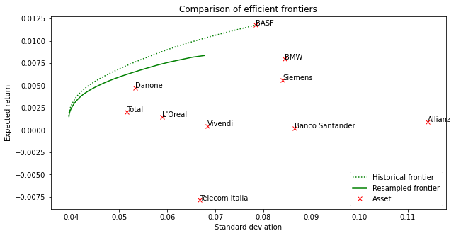

Evidently, the simulated efficient frontier lies below the classical one. Why?

If we take a particular Monte Carlo draw, say \(\theta_i\), and plot its associated frontier, that frontier may lie either to the right or to the left of the original one. At discrete points along the frontier, we record the portfolio weights. We then average these weights (not the frontiers themselves) and apply the resulting average weights to the original \(\theta\).

We know that the optimal (efficient) portfolio weights given \(\theta\) are \(a_K\). If we instead apply \(a^*_K\) to \(\theta\), the resulting frontier must therefore lie to the right of the original one. In other words, if \(a_K\) is efficient for \(\theta\), then \(a^*_K\) cannot also be efficient for \(\theta\). Although each simulated efficient frontier is efficient with respect to its own simulated \(\mu_i\) and \(\Sigma_i\), it is inefficient with respect to the original historical estimates \(\mu\) and \(\Sigma\). A resampled portfolio is therefore, by definition, no longer efficient for \(\theta\), but it does account for the estimation risk around the true \(\theta\).

We now plot the portfolio weights associated with the efficient frontiers as a bar chart:

1. Resampled efficient frontier

fig2 = plt.figure(num=2, facecolor='w', figsize=(10, 5))
plt.stackplot(S_Return*12, S_Weight.T*100) # annualised returns
plt.axis([np.min(S_Return*12), np.max(S_Return*12), 0.0, 100.0])
plt.legend(list(frame1.columns),
           loc='upper left', bbox_to_anchor=(1.0, 1.0), frameon=False)
plt.xlabel('Target expected return')
plt.ylabel('Allocation weight (%)')
plt.title('Portfolioweights for the resampled efficient frontier')
plt.show()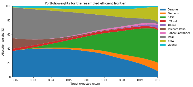

2. Classical efficient frontier based on simple history-based estimation

fig3 = plt.figure(num=3, facecolor='w', figsize=(10, 5))
plt.stackplot(V_Target*12, V_Weight.T*100)
plt.axis([np.min(V_Target*12), np.max(V_Target*12), 0.0, 100.0]) # annualised return
plt.legend(list(frame1.columns),
           loc='upper left', bbox_to_anchor=(1.0, 1.0), frameon=False)
plt.xlabel('Target expected return')
plt.ylabel('Allocation weight (%)')
plt.title('Portfolioweights for the historic efficient frontier')
plt.show()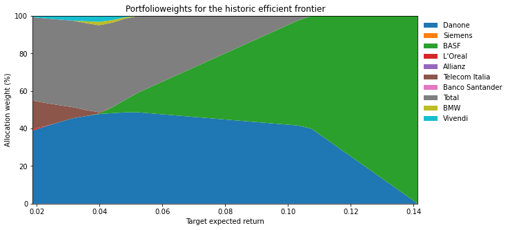

Comparing the charts shows that, under portfolio resampling, markedly more securities enter the portfolio, allowing greater diversification. Abrupt shifts in individual securities’ weights are also less pronounced, so the portfolio composition is more diversified and more stable overall. This stability comes from averaging the portfolio weights, so that small changes in the inputs now produce only small changes in the optimized portfolios.

6.3.3 Excursus: Comparison of simulated vs. historical means and variances/covariances

We simulate (i.e. draw random realizations from) a multivariate normal distribution. As the number of draws (size) increases, the simulated moments approach the distribution’s true moments \(\mu\) and \(\Sigma\).

np.random.seed(32)
df = pd.DataFrame(np.asarray(np.random.multivariate_normal(means_hist,\
                Sigma_hist, size = 50000)), columns=frame1.columns)
pd.DataFrame({'sim': df.mean().values, 'hist.': means_hist,\
             'difference':df.mean().values-means_hist}, \
             index=frame1.columns)

	sim	hist.	difference
Danone	0.004407	0.004711	-0.000304
Siemens	0.004495	0.005585	-0.001090
BASF	0.010784	0.011778	-0.000994
L'Oreal	0.000882	0.001505	-0.000623
Allianz	-0.000273	0.000947	-0.001220
Telecom Italia	-0.007887	-0.007870	-0.000017
Banco Santander	-0.000349	0.000191	-0.000540
Total	0.001659	0.002032	-0.000373
BMW	0.006899	0.007962	-0.001063
Vivendi	-0.000316	0.000421	-0.000737

6.3.4 Graphical representation of the historical and the \(M\) simulated efficient frontiers

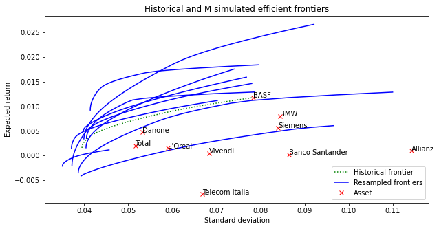
Finally, we plot the original efficient frontier together with the \(M\) simulated efficient frontiers.

To this end we create two lists: list_Risk for the portfolio variance and list_Target for the expected portfolio return. Each list will ultimately hold \((1+M)\) elements (each a 1-D array of dimension \(K\)), since every efficient frontier consists of \(K\) points.

First we compute the historical efficient frontier via ef_front and append the 1-D (dimension K) arrays Risk (for \(\sigma^2_P\)) and Target (for \(\mu_P\)) to the two lists. Then, for \(i=1,..., M\), we simulate the input parameters \(\theta_i=\{\mu_i, \Sigma_i\}\) under the assumption of a multivariate normal distribution for the return vector and compute the \(M\) efficient frontiers, again appending the two arrays describing each frontier (\(\mu_{P,i}\) and \(\sigma^2_{P,i}\)) to the lists.

Finally, both lists are converted into arrays (i.e. \((M+1)xK\) matrices) and returned by the function.

# function returns two lists with (1+M) elements; 
# each element is a 1-D array of dimension K;
# K is the number of points on the ef: K different target 
# expected portfolio returns and portfolio return std's
def resampled_frontiers(M, means_hist, Sigma_hist):
# M: number of Monte Carlo runs   
    np.random.seed(42)
    list_Risk = []
    list_Target = []
    # first, calculate the historical ef 
    _, Risk, Target = ef_front(means_hist, Sigma_hist)
    # and append to the two lists
    list_Risk.append(Risk)
    list_Target.append(Target)
    # now, calculate the M simulated ef's
    for i in range(M):
        df = pd.DataFrame(np.asarray(np.random.multivariate_normal(means_hist,\
                Sigma_hist, size = 110)), columns=frame1.columns)
        means = df.mean().values
        Sigma = df.cov().values
        # ef_front returns: weights, risk, target return! 
        _, Risk, Target = ef_front(means, Sigma)
        # and append to the lists
        list_Risk.append(Risk)
        list_Target.append(Target)
    list_Risk = np.array(list_Risk)
    list_Target = np.array(list_Target)
    return list_Risk, list_Target 

The following function draw_efs plots the historical efficient frontier together with the \(M\) simulated ones, using the two arrays returned by resampled_frontiers.

def draw_efs(M, means_hist, Sigma_hist):
    Risk, Target = resampled_frontiers(M, means_hist, Sigma_hist)

    fig1 = plt.figure(num=1, facecolor='w', figsize=(10, 5))
    ax = fig1.add_subplot(111)
    plt.plot(Risk[0,:], Target[0,:], 'g:', label='Historical frontier')
    plt.plot(Risk[1,:], Target[1,:], 'b-', label='Resampled frontiers')
    for i in range(2,M+1):
        plt.plot(Risk[i,:], Target[i,:], 'b-')
    plt.plot(np.sqrt(np.diagonal(Sigma_hist)), means_hist, 'rx', label='Asset')
    for i, txt in enumerate(frame1.columns):
        ax.annotate(txt, (np.sqrt(np.diagonal(Sigma_hist))[i],means_hist[i]))
    plt.legend(loc=4,  frameon=True)
    plt.xlabel('Standard deviation')
    plt.ylabel('Expected return')
    plt.title('Historical and M simulated efficient frontiers')
    return plt.show()

To conclude, let us plot ten simulated efficient frontiers together with the historical one.

draw_efs(10, means_hist, Sigma_hist)

6.4 Summary

In this chapter you have deepened your understanding of estimation risk in portfolio optimization and its effects on the optimal portfolio weights. You can explain the principle of Michaud’s portfolio resampling and follow how simulated return and covariance estimates are used to reduce instability. You are now able to implement resampling procedures in Python — running repeated optimizations on random samples and aggregating the results — and to compare resampling-based portfolios with classical Markowitz portfolios, evaluating the differences systematically in terms of stability, diversification, and robustness. This enables you to apply portfolio resampling critically and reflectively as a practice-oriented way of accounting for uncertainty in the input parameters.

6.5 Further reading and references

• Michaud, R.O, Michaud, R.O., (2008). Efficient Asset Management: A Practical Guide to Stock Portfolio Optimization and Asset Allocation, 2nd Edition, Oxford University Press.

Go deeper

Experience this chapter in the live seminar

In the in-house seminar Quant Portfolio Management, you will work through these methods hands-on in Python — with personal feedback, tailored case studies, and direct exchange with Prof. Dr. Thomas Mählmann.

Learn more about the seminar →