After completing this chapter, you will be able to …
explain the core idea behind risk-based portfolio approaches and justify why these methods deliberately avoid explicitly estimating expected returns.
classify alternative portfolio approaches—such as minimum-variance, equal-risk-contribution, and diversification-based strategies—in technical terms and explain their objectives within quantitative portfolio management.
use Python to compute risk and covariance measures from historical return data and use these as the key inputs for risk-based portfolio optimization.
implement risk-based portfolios in practice with suitable Python libraries and analyze and compare their properties.
critically assess the strengths and weaknesses of risk-based portfolio approaches and give a clear rationale for how they can be applied in professional portfolio and risk management.
7.2 Introduction and motivation
We have already seen that the traditional arithmetic-mean estimator yields only very imprecise estimates of expected returns. Errors in these estimates are especially problematic, as they tend to produce extreme, suboptimal portfolio weights; indeed, the classical mean-variance approach alone frequently leads to portfolios with extreme weights. One way to alleviate this problem is to abandon the estimation of expected returns in portfolio construction altogether. This brings us to the risk-based approaches (also known as risk-balancing approaches) to asset allocation. Rather than seeking the optimal trade-off between a portfolio’s target return and its risk, risk-based portfolio construction focuses on how risk is allocated across the assets in the portfolio.
Beyond addressing the estimation-error problem, weighting asset classes according to the risk they contribute also makes sense in light of the 2008-2009 financial crisis. During that period, even well-diversified portfolios sometimes suffered heavy losses and large swings in value. As a result, the benefits of diversification are now viewed more skeptically, because diversification proves weaker in times of crisis, when correlations rise. The diversification benefit also appears limited as more asset classes are added to a portfolio, at least when those additional asset classes are illiquid and lack transparency, since they can introduce further, undesirable risks.
Against this backdrop—and given how unreliable long-term return forecasts have proven to be—allocation frameworks were developed that rely not on forecasts of expected returns but solely on assumptions about volatilities and correlations. The asset allocation is thus driven by risk: the weight of an asset class can be reduced, for example, whenever its volatility or its correlation with another asset class increases.
One such framework is the risk parity approach. Its aim is to balance the risk contributed by each asset class as evenly as possible, so that no single asset class (equities, say) can drag down the entire portfolio. The risk parity approach comes in two variants: the equal-risk-budget (ERB) strategy and the equal-risk-contribution (ERC) strategy. Other risk-based allocation concepts include the global-minimum-variance approach and the maximum-diversification approach, though these two do not directly target equal risk budgets or risk contributions. A final way to balance risk is to build a “naive” portfolio that weights all asset classes equally (the equally-weighted approach).
The remainder of the chapter proceeds as follows. We first cover the fundamentals of the risk parity approach and then present the equal-risk-budget (ERB) and equal-risk-contribution (ERC) strategies. Next, we introduce the alternative risk-balancing concepts—the equally-weighted, global-minimum-variance, and maximum-diversification approaches. Finally, a case study provides a comparative analysis of all five approaches.
7.3 The risk parity approach
7.3.1 Fundamentals
A traditional capital-based split—say, 50% equities and 50% bonds—can leave the portfolio’s return and risk dominated by equities, with the bonds contributing little. In effect, the portfolio is not truly diversified. The risk parity approach, by contrast, allocates considerably less to equities and more to other asset classes than a traditional allocation would. If both asset classes in an equity/bond portfolio are to contribute equally to total risk (a risk-balanced portfolio), equities must be held at a smaller weight in favor of bonds. This spreads the portfolio’s risk budget more broadly across other investments, and the resulting portfolio returns can be expected to display lower volatility.
Unlike asset allocation based on portfolio theory, for instance, the risk parity approach requires no forecasts of expected returns. It does, however, still require estimates of risk measures and—depending on the variant—correlations. Correlations are not needed for the equal-risk-budget (ERB) strategy, the first variant of the risk parity approach, because it weights each investment according to its inverse volatility. The second variant, the equal-risk-contribution (ERC) strategy, does require correlation estimates.
We begin with the following definition.
Definition: A portfolio that satisfies the condition
\[\begin{equation*}
w_1\partial_1\sigma_p = \cdots = w_N\partial_N\sigma_p,\quad
\sigma_p=\sqrt{w\Sigma w^{T}},\quad
\partial_n\sigma_p = \frac{\partial\sigma_p}{\partial w_n},
\end{equation*}\] is called a risk parity portfolio.
The underlying idea is to achieve an equal—or, more generally, a specific target—risk budget across all investments in the portfolio. Various risk measures can be used; here we restrict ourselves to the standard deviation \(\sigma\). Risk parity requires each asset to contribute equally to the portfolio’s total volatility, which is enforced by setting the risk contribution (RC) of all assets equal. The expression \(\frac{\partial\sigma_p}{\partial w_n}\) denotes the marginal risk contribution (MRC) of the n-th asset: it measures the additional portfolio risk generated by an infinitesimal increase in that asset’s weight and is formally defined as the derivative of the portfolio return’s standard deviation \(\sigma_p\) with respect to the weight \(w_n\). The RC, in turn, is the product of the asset’s weight and its MRC. The following relationships therefore hold.
The standard deviation of the portfolio return \(r_p\) is given by (note that \(w\) is a row vector):
In other words, the MRC is obtained by multiplying the variance-covariance matrix of the asset returns by the weight vector row by row and summing. The n-th element of the (Nx1) vector \(\Sigma w^{T}\), scaled by the portfolio standard deviation, then gives the marginal risk contribution of the n-th asset.
where \(\beta_n=\) the beta factor of the n-th asset relative to the portfolio return.
7.3.2 Equal-risk-budget (ERB) strategy
This strategy aims to make the risk budgets of all investments in the portfolio identical—a simplification of the general risk parity definition given above. Taking the standard deviation as the risk measure, an investment’s risk budget is defined as the product of its standard deviation and its portfolio weight. Unlike the risk contributions, this ignores the correlations between investments; equivalently, all asset returns are assumed to have identical correlations with the portfolio return. For the ERB approach, then—departing slightly from the definition above—the objective for all investments 1 to N is (note that the risk budget, the product of standard deviation and portfolio weight, can be read as the risk contribution under perfect correlation):
Under the ERB strategy, the asset weights are therefore inversely proportional to their volatilities.
7.3.3 Equal-risk-contribution (ERC) strategy
The equal-risk-contribution (ERC) strategy aims to equalize the individual assets’ risk contributions to the portfolio’s total risk \((\sigma_p)\). This matches exactly the risk parity definition given in the Fundamentals section. As shown above, the absolute risk contribution of an asset n to total risk can be written as:
\[ MRC_n= \frac{(\Sigma w^{T})_{n}}{\sigma_p} \]
The vector of marginal risk contributions \(\partial_{n}\sigma_p\) across all assets is therefore:
We also noted earlier that the RCs sum to total risk \((\sigma_p)\) and that the RC of an asset n equals its MRC weighted by \(w_n\). Hence, for all RCs to be equal, we must have:
Since the absolute risk contributions in the ERC portfolio are identical, so too are the relative risk contributions \((RC/\sigma_p)\) of the N assets. It follows (see equation (3) above) that:
\[ \textrm{Relative risk contribution in the ERC portfolio} = w^{ERC}_n \cdot \frac{Cov(r_n,r_p)}{\sigma^2_p}=w^{ERC}_n \cdot \beta^{ERC}_n=\frac{1}{N},\]
where \(\beta^{ERC}_n=\) the beta factor of asset n relative to the ERC portfolio. The weight \(w^{ERC}_n\) can then also be expressed as:
\[ w^{ERC}_n=\frac{1}{N \cdot \beta^{ERC}_n}, \quad \text{where for an ERC portfolio it holds that:} \quad \Sigma^N_{n=1}w^{ERC}_n=1. \]
An asset’s weight is therefore inversely proportional to its beta factor: the higher the beta, the lower the weight in the portfolio, and vice versa. Accordingly, assets with a high (low) standard deviation or a high (low) correlation with the portfolio return receive a lower (higher) weight.
7.4 Alternative risk-based approaches
The risk parity approach should be distinguished from other methods that likewise avoid estimating returns for asset allocation. Chief among these is the global-minimum-variance approach, which identifies the risk-minimizing combination of the available investments. The maximum-diversification approach is another risk-based allocation concept. Finally, the equally-weighted strategy—best described as a “naive” approach—serves as a benchmark for comparison.
7.4.1 Equally-weighted (EW) approach
The equally-weighted approach is arguably the simplest form of diversification, since each of the N assets in the portfolio receives the weight:
\[ w^{EW}_n=\frac{1}{N} \]
Here, neither the type of investment nor which asset classes are included matters, and the same is true of the assets’ return and risk characteristics. This strategy is therefore best used only as a benchmark for evaluating the performance of asset allocation strategies. As noted above, the ERC approach, for instance, reduces to an equally weighted allocation only in the special case where the assets have identical correlations and equal standard deviations. When risks are distributed unevenly across a portfolio, however, the equally-weighted approach ultimately concentrates risk, because every asset—whether the riskiest or the least risky—receives the same weight.
7.4.2 Global-minimum-variance (GMV) approach
The global-minimum-variance approach follows from portfolio theory: it seeks the efficient portfolio with the lowest possible risk. This global-minimum-variance portfolio is found by taking the partial derivative of the portfolio-variance function with respect to each asset weight \((w_n)\) and setting it to zero: \(\frac{\partial{\sigma^2_p}}{\partial{w_n}}\)
Case 1: closed-form solution
The GMVP weights can be determined analytically as long as there are no inequality constraints, such as a ban on short selling or position limits. In that case the weights solve the following minimization problem:
Note that \(w^{GMV}\) does not depend on the vector of expected returns \(\mu\); the GMVP can therefore be determined without knowing \(\mu\).
Case 2: numerical solution
In practice, investment restrictions often prevent many institutional investors from taking short positions. To reflect this, a non-negativity constraint on the weights must be added to the optimization problem, and a closed-form solution is then no longer available.
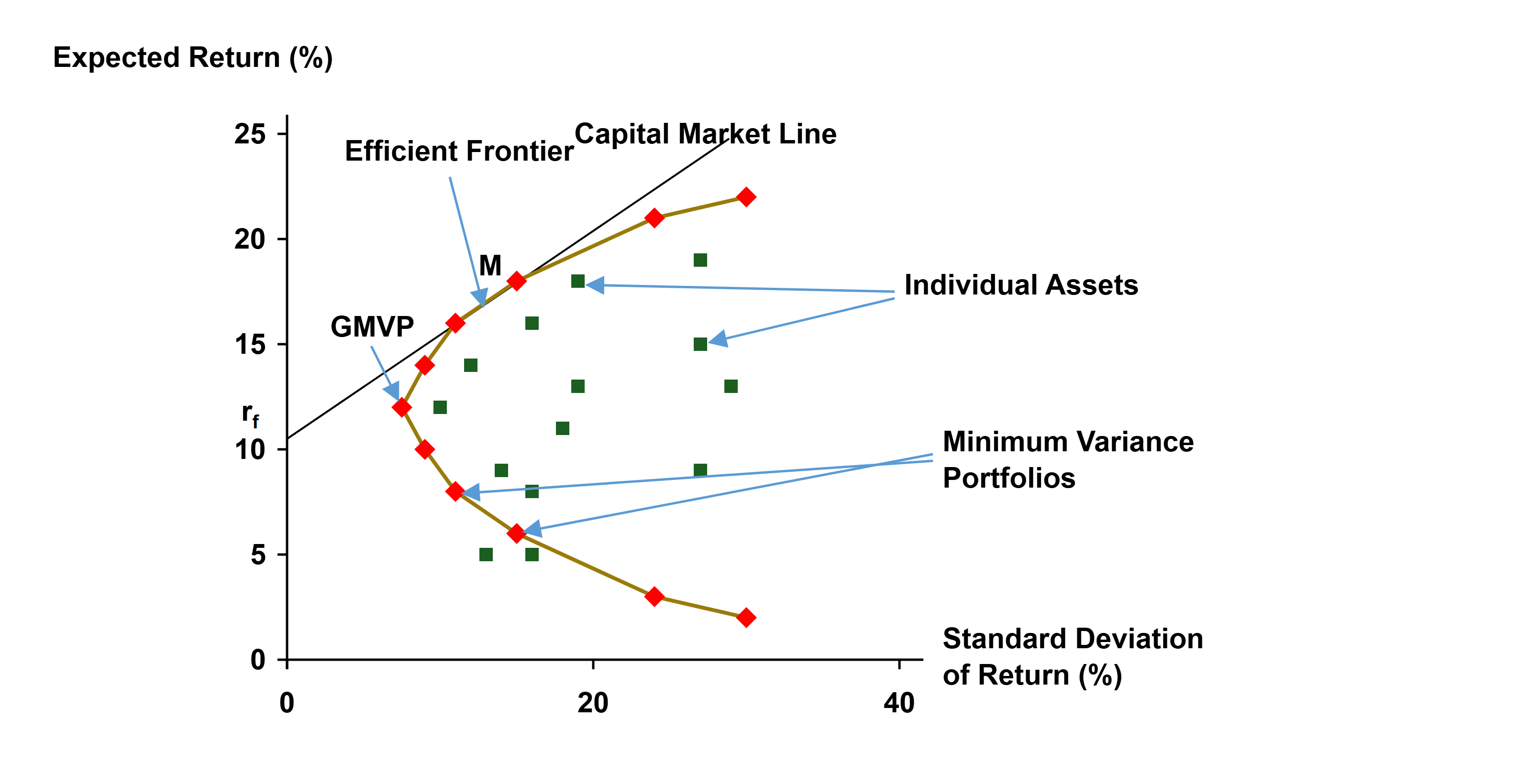
Graphically, the GMV portfolio can be located as shown in the following figure.
The figure shows that, in risk-return terms, portfolios on the capital market line are more efficient than the GMVP. If, for instance, total portfolio risk is to equal that of the GMVP, the same risk can also be achieved by combining the market portfolio M with the risk-free asset \(r_f\)—but with a higher expected return.
7.4.3 Maximum-diversification (MD) approach
To maximize a portfolio’s diversification, one can use the maximum-diversification approach, also known as the “most-diversified” approach. The diversification is quantified by the diversification ratio (DR) (see Choueifaty et al., 2013):
The numerator of the diversification ratio is the weighted average of the individual assets’ standard deviations, while the denominator is the portfolio’s standard deviation. For a long-only portfolio (no short selling) with \(\sigma_n>0\) for at least one investment, we have \(DR\geq 1.\) If every pairwise correlation equals 1, the numerator and denominator coincide; otherwise, the diversification effect makes the denominator smaller than the numerator. The diversification ratio thus measures the diversification benefit obtained from investments that are not perfectly correlated. In essence, it maximizes the gap between two volatility measures of the same portfolio: the numerator is the portfolio risk that would prevail without diversification, and the denominator is the (actual) risk with diversification.
The maximum-diversification (MD) portfolio is the one that maximizes the diversification ratio:
Adding further constraints (e.g. position limits or the long-only constraint) requires numerical optimization.
For the resulting portfolio, one can show that every investment with a weight \(w_n>0\) has the same (positive) correlation with the MD portfolio. In this case the correlation between any portfolio P and the MD portfolio can be written as the ratio of their diversification ratios (Choueifaty and Coignard, 2008, p. 42):
\[ Corr(r_p, r_{MD})=\frac{DR_p}{DR_{MD}}, \]
with
\[DR_p=\textrm{Diversification ratio of portfolio P} \]\[DR_{MD}=\textrm{Diversification ratio of the maximum-diversification portfolio} \]
A portfolio consisting of a single investment n has a diversification ratio of 1, so for every investment n held in the maximum-diversification portfolio:
The ratio of \(MRC_n\) to \(\sigma_n\) can be interpreted as the “relative” or “scaled” marginal volatility (cf. Demey et al., 2010, p. 14, and Roncalli, 2014, p. 173).
7.5 Case study
We now examine the strategies presented above more closely using an example portfolio of four assets: A, B, C, and D. The standard deviations and the correlations between the individual asset returns are given by the example data Stdev and CorrMatrix below:
Code
import pandas as pdimport numpy as npimport numpy.linalg as lafrom scipy.optimize import minimizeTOLERANCE =1e-15import warnings# Ignore all warningswarnings.filterwarnings("ignore")Stdev = np.array([0.18, 0.11, 0.16, 0.24])CorrMatrix = np.array([[1.00, 0.40, -0.10, 0.30], [0.40, 1.00, 0.10, 0.20], [-0.10, 0.10, 1.00, -0.15], [0.30, 0.20, -0.15, 1.00]])
From these, the following covariances can be derived.
We begin with the equal-risk-budget strategy. The weights are inversely proportional to the asset volatilities, \(w^{ERB}_n=\frac{1/\sigma_n}{\Sigma^N_{j=1}1/\sigma_j}\), and the risk budget is defined as the product of an asset’s return standard deviation and its weight. The following table shows how the individual asset weights \(w_n\) in the ERB portfolio are obtained.
These values show that higher-risk (lower-risk) assets are underweighted (overweighted). The allocation therefore tilts toward lower-risk assets, which also tend to have a relatively low beta.
The risk budget—the standard deviation weighted by the portfolio weight—thus equals 3.9899% for every investment. Using these values, we can compute the weighted variance-covariance matrix (\(w^{T}\Sigma w\)).
The variance of the ERB portfolio can be read off the table; in this example it is 0.0087557, giving an ERB portfolio standard deviation of 9.3572%:
\[ \sigma_{ERB}=\sqrt{0.0087557}=9.35720\%.\]
The table below reports the absolute risk contributions (RC), the relative risk contributions (rRC), the covariances of each asset return with the portfolio return, the beta factors relative to the ERB portfolio, and the marginal risk contributions (MRC), computed using formulas (1)-(3) from the Fundamentals section:
Code
# calculation of the absolute risk contribution: formulas (1) and (2)rc=np.zeros(4)for i inrange(4): rc[i]=(weight_erb[i]*Sigma[i,:]*np.asmatrix(weight_erb).T)/0.093572# calculation of the relative risk contributionrrc=np.zeros(4)for i inrange(4): rrc[i]=rc[i]/np.sum(rc)# calculation of the covariance of the asset return with the portfolio return: formula (3)cov_ri_rp=np.zeros(4)for i inrange(4): cov_ri_rp[i]=Sigma[i,:]*np.asmatrix(weight_erb).T# calculation of the beta of the asset return with the portfolio returnbeta_ri=np.zeros(4)for i inrange(4): beta_ri[i]=cov_ri_rp[i]/0.093572**2# and now the marginal risk contributionmrc=np.zeros(4)for i inrange(4): mrc[i]=rc[i]/weight_erb[i]# Finally we present the results for the ERB strategy# clearly in a tableresults_erb=pd.DataFrame({'absolute RC (%)': np.round(rc*100,4), \'relative RC (%)': np.round(rrc*100,4),'Cov(r_i,r_p)':np.round(cov_ri_rp,4),'Beta': np.round(beta_ri,4),'MRC (%)': np.round(mrc*100,4)},index=Assets) results_erb.loc['Total', results_erb.columns[:2]] = results_erb.iloc[:, :2].sum(axis=0)results_erb
absolute RC (%)
relative RC (%)
Cov(r_i,r_p)
Beta
MRC (%)
A
2.7221
29.0909
0.0115
1.3124
12.2804
B
2.8922
30.9091
0.0075
0.8521
7.9737
C
1.4461
15.4545
0.0054
0.6197
5.7991
D
2.2968
24.5455
0.0129
1.4764
13.8154
Total
9.3572
100.0000
NaN
NaN
NaN
The table shows that the individual assets have different risk contributions. These differences arise because the asset weights are set without regard to the correlations between the assets’ returns; diversification effects therefore play no role in determining the weights, even though they do show up in the results in the table.
This confirms that the weighted betas equal the relative risk contributions.
7.5.2 Equal-risk-contribution strategy
We now implement the ERC strategy on the example data. To find the optimal ERC weights numerically with scipy.optimize, we define three functions: - calulate_portfolio_var computes the variance of the portfolio return \(\sigma^2_p\) - calculate_risk_contribution computes the vector of risk contributions, \(w_n\frac{(\Sigma w^{T})_n}{\sigma_p} \quad \text{for}\quad n=1, ..., N\) - risk_contribution_objective implements the objective function of the general minimization problem in equation (5)
The constraints are the budget constraint the long-only condition: the weights must lie between 0 and 1 and sum to 1.
Code
# ERC optimization: definition of required functionsdef calculate_portfolio_var(w,Sigma):# function to calculate the portfolio return variance w = np.matrix(w) # w is a row vector!return (w*Sigma*w.T)[0,0]def calculate_risk_contribution(w,Sigma):# function to calculate the risk contribution w = np.matrix(w) sigma_p = np.sqrt(calculate_portfolio_var(w,Sigma))# marginal risk contribution MRC = Sigma*w.T# risk contribution RC = np.multiply(MRC,w.T)/sigma_preturn RCdef risk_contribution_objective(x,pars):# x denotes the vector of the sought portfolio weights# the variance-covariance matrix is the first component of the array of given parameters Sigma = pars[0]# the second component contains the target risk allocation x_t = pars[1] sig_p = np.sqrt(calculate_portfolio_var(x,Sigma)) # portfolio risk risk_target = np.asmatrix(np.multiply(sig_p,x_t)) asset_RC = calculate_risk_contribution(x,Sigma) J =sum(np.square(asset_RC-risk_target.T))[0,0] # sum of the squared errorsreturn Jdef total_weight_constraint(x):return np.sum(x)-1.0def long_only_constraint(x):return xx_t = [0.25, 0.25, 0.25, 0.25] # target risk allocation as a percentage of total riskweight_ew = np.tile(1.0/4, 4) # equal weighting as starting vector# constraints of the optimizationcons = ({'type': 'eq', 'fun': total_weight_constraint},{'type': 'ineq', 'fun': long_only_constraint})# optimizationres= minimize(risk_contribution_objective, weight_ew, args=[Sigma,x_t], method='SLSQP',tol=TOLERANCE,constraints=cons, options={'disp': False})weight_erc = np.array(res.x)
We can also wrap everything into a single, elegant function:
Code
#### An elegant function for the entire optimization process:def get_risk_parity_weights(covariances, assets_risk_budget, initial_weights):# constraints of the optimization: only long positions that in total# sum to 100% constraints = ({'type': 'eq', 'fun': lambda x: np.sum(x) -1.0}, {'type': 'ineq', 'fun': lambda x: x})# optimization with scipy optimize_result = minimize(fun=risk_contribution_objective, x0=initial_weights, args=[covariances, assets_risk_budget], method='SLSQP', constraints=constraints, tol=TOLERANCE, options={'disp': False})# extracting the weights from the output of the optimization weights = optimize_result.x# the function returns the desired optimal weightsreturn weights
The ERC portfolio again tends to underweight (overweight) higher-risk (lower-risk) investments—though this is not a general rule, since the correlations among the investments also come into play. Broadly speaking, the ERC strategy, too, tilts toward lower-risk investments. For this example, the weighted variance-covariance matrix is as follows.
The weighted variance-covariance matrix gives an ERC portfolio variance of 0.0085744, corresponding to a portfolio standard deviation of 9.25984%: \(\sigma_p=\sqrt{0.0085744}=9.25984\%\).
As for the ERB strategy, we can tabulate the absolute risk contributions (RC), the relative risk contributions, the covariances of each investment return with the portfolio return, the beta factors relative to the ERC portfolio, and the marginal risk contributions:
Code
# calculation of the absolute risk contribution: formulas (1) and (2)rc=np.zeros(4)for i inrange(4): rc[i]=(weight_erc[i]*Sigma[i,:]*np.asmatrix(weight_erc).T)/0.0925984# calculation of the relative risk contributionrrc=np.zeros(4)for i inrange(4): rrc[i]=rc[i]/np.sum(rc)# calculation of the covariance of the asset return with the portfolio return: formula (3)cov_ri_rp=np.zeros(4)for i inrange(4): cov_ri_rp[i]=Sigma[i,:]*np.asmatrix(weight_erc).T# calculation of the beta of the asset return with the portfolio returnbeta_ri=np.zeros(4)for i inrange(4): beta_ri[i]=cov_ri_rp[i]/0.0925984**2# and now the marginal risk contributionmrc=np.zeros(4)for i inrange(4): mrc[i]=rc[i]/weight_erc[i]# Finally we present the results for the ERC strategy# clearly in a tableresults_erc=pd.DataFrame({'absolute RC (%)': np.round(rc*100,4), \'relative RC (%)': np.round(rrc*100,4),'Cov(r_i,r_p)':np.round(cov_ri_rp,4),'Beta': np.round(beta_ri,4),'MRC (%)': np.round(mrc*100,4)},index=Assets) results_erc.loc['Total', results_erc.columns[:2]] = results_erc.iloc[:, :2].sum(axis=0)results_erc
absolute RC (%)
relative RC (%)
Cov(r_i,r_p)
Beta
MRC (%)
A
2.315
25.0
0.0105
1.2195
11.2920
B
2.315
25.0
0.0069
0.8001
7.4086
C
2.315
25.0
0.0069
0.8058
7.4617
D
2.315
25.0
0.0124
1.4512
13.4375
Total
9.260
100.0
NaN
NaN
NaN
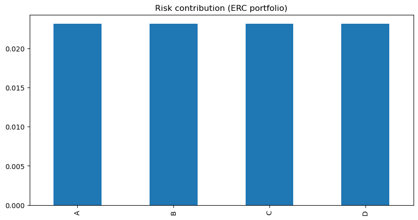
The table shows that all assets have the same risk contribution, exactly as the ERC strategy intends.
This example makes clear that the individual investments’ beta factors differ from those in the ERB portfolio. The reason is the difference between the ERB and ERC portfolios, which stems from the fact that the ERB weights are set without accounting for the correlations between the assets’ returns.
The example also shows that all weighted beta factors in the ERC portfolio are equal, so that:
For this reason, the ERC portfolio is sometimes called a beta parity portfolio, while the ERB portfolio is called a volatility parity portfolio.
Relationship between the ERB and ERC portfolios
When all asset classes have identical correlations, and also in the two-asset case, the equal-risk-contribution approach reduces to the equal-risk-budget approach (cf. Maillard et al., 2009).
Suppose, for instance, that in the example above all correlations between the investments equal 0.2. This gives the following results:
These weights match those of the ERB approach. Note that the changed correlations produce a different portfolio return standard deviation (10.0938%) than the ERB value in the base example; under identical correlations, however, this standard deviation is the same for both portfolios (ERB and ERC).
If we additionally assume that all assets have identical volatilities, both approaches yield an equally weighted portfolio.
7.5.3 Equally-weighted strategy
In our four-asset example, each weight \(w^{EW}_n\) is 25%. These weights produce the weighted variance-covariance matrix shown in the following table.
The weighted variance-covariance matrix gives an EW portfolio variance of 0.0103913, corresponding to a portfolio standard deviation of 10.19375%: \(\sigma_p=\sqrt{0.01039125}=10.19375\%.\)
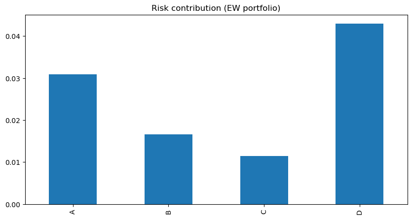
Clearly, equal weights do not imply equal risk contributions.
The following table reports the absolute risk contributions (RC), the relative risk contributions, the covariances of each investment return with the portfolio return, the beta factors relative to the EW portfolio, and the marginal risk contributions:
Code
# calculation of the absolute risk contribution: formulas (1) and (2)rc=np.zeros(4)for i inrange(4): rc[i]=(weight_ew[i]*Sigma[i,:]*np.asmatrix(weight_ew).T)/0.1019375# calculation of the relative risk contributionrrc=np.zeros(4)for i inrange(4): rrc[i]=rc[i]/np.sum(rc)# calculation of the covariance of the asset return with the portfolio return: formula (3)cov_ri_rp=np.zeros(4)for i inrange(4): cov_ri_rp[i]=Sigma[i,:]*np.asmatrix(weight_ew).T# calculation of the beta of the asset return with the portfolio returnbeta_ri=np.zeros(4)for i inrange(4): beta_ri[i]=cov_ri_rp[i]/0.1019375**2# and now the marginal risk contributionmrc=np.zeros(4)for i inrange(4): mrc[i]=rc[i]/weight_ew[i]# Finally we present the results for the EW strategy# clearly in a tableresults_ew=pd.DataFrame({'absolute RC (%)': np.round(rc*100,4), \'relative RC (%)': np.round(rrc*100,4),'Cov(r_i,r_p)':np.round(cov_ri_rp,4),'Beta': np.round(beta_ri,4),'MRC (%)': np.round(mrc*100,4)},index=Assets) results_ew.loc['Total', results_ew.columns[:2]] = results_ew.iloc[:, :2].sum(axis=0)results_ew
absolute RC (%)
relative RC (%)
Cov(r_i,r_p)
Beta
MRC (%)
A
3.0901
30.3140
0.0126
1.2126
12.3605
B
1.6591
16.2757
0.0068
0.6510
6.6364
C
1.1478
11.2595
0.0047
0.4504
4.5910
D
4.2968
42.1508
0.0175
1.6860
17.1870
Total
10.1938
100.0000
NaN
NaN
NaN
As a result, assets A and D—the two riskiest assets—together account for over 72% of total risk, and the overall portfolio risk is higher than under the risk parity approaches.
7.5.4 Global-minimum-variance strategy
For the example portfolio of assets A, B, C, and D, and in the absence of any short-selling ban (or other inequality constraints), formula (6) gives the following GMVP weights.
Code
iota = np.ones(Sigma.shape[0]) # creates a unit vector of dimension 4inv_Sigma = la.inv(Sigma) # inverse of the variance-covariance matrixweight_gmv = inv_Sigma @ iota / (iota @ inv_Sigma @ iota)weight_gmv
In this example, an asset’s portfolio weight decreases as its risk increases. As with the risk parity approach, the allocation therefore tilts toward lower-risk assets—though, again, this is not a general rule, since the correlations among the assets must also be taken into account. These weights produce the weighted variance-covariance matrix shown in the following table.
The weighted variance-covariance matrix gives a GMVP variance of 0.0078135, corresponding to a portfolio standard deviation of 8.83941%:
\[\sigma_p=\sqrt{0.0078135}=8.83941\%.\]
As with the risk parity approach, we can tabulate the GMVP’s absolute risk contributions (RC), relative risk contributions, the covariances of each investment return with the portfolio return, the beta factors relative to the GMV portfolio, and the marginal risk contributions:
Code
# calculation of the absolute risk contribution: formulas (1) and (2)rc=np.zeros(4)for i inrange(4): rc[i]=(weight_gmv[i]*Sigma[i,:]*np.asmatrix(weight_gmv).T)/0.0883941# calculation of the relative risk contributionrrc=np.zeros(4)for i inrange(4): rrc[i]=rc[i]/np.sum(rc)# calculation of the covariance of the asset return with the portfolio return: formula (3)cov_ri_rp=np.zeros(4)for i inrange(4): cov_ri_rp[i]=Sigma[i,:]*np.asmatrix(weight_gmv).T# calculation of the beta of the asset return with the portfolio returnbeta_ri=np.zeros(4)for i inrange(4): beta_ri[i]=cov_ri_rp[i]/0.0883941**2# and now the marginal risk contributionmrc=np.zeros(4)for i inrange(4): mrc[i]=rc[i]/weight_gmv[i]# Finally we present the results for the GMV strategy# clearly in a tableresults_gmv=pd.DataFrame({'absolute RC (%)': np.round(rc*100,4), \'relative RC (%)': np.round(rrc*100,4),'Cov(r_i,r_p)':np.round(cov_ri_rp,4),'Beta': np.round(beta_ri,4),'MRC (%)': np.round(mrc*100,4)},index=Assets) results_gmv.loc['Total', results_gmv.columns[:2]] = results_gmv.iloc[:, :2].sum(axis=0)results_gmv
absolute RC (%)
relative RC (%)
Cov(r_i,r_p)
Beta
MRC (%)
A
0.9788
11.0728
0.0078
1.0
8.8394
B
4.3008
48.6549
0.0078
1.0
8.8394
C
2.7047
30.5987
0.0078
1.0
8.8394
D
0.8551
9.6736
0.0078
1.0
8.8394
Total
8.8394
100.0000
NaN
NaN
NaN
The first striking feature of the table is that every asset’s return has the same covariance with the GMVP return. This can also be shown analytically. For an arbitrary investment Z, the variance of a portfolio combining the GMVP and Z is:
Because any change in the weights \(w_n\) would raise the portfolio variance above that of the GMV portfolio, we immediately have \(w_{GMV}=100\%\) and \(w_Z=0\%\). This in turn yields (see Kleeberg, 1995, p. 17ff.):
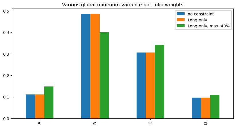
The covariance of the GMVP with any investment Z thus equals the GMVP’s variance. If additional constraints apply when determining the GMVP—such as a cap on individual weights (see above) or the long-only constraint—this equality between the GMVP variance and its covariance with any other investment Z may no longer hold.
Because covariance and variance coincide in this way, every investment in the portfolio also has a beta factor (relative to the GMVP) of 1:
The marginal risk contribution is likewise identical for all GMVP assets and equals the GMVP’s standard deviation, as follows from the formal definition of the marginal risk contribution (MRC) given earlier:
The absolute risk contribution (RC) of each investment n is, in general, \(RC_n=w_n \cdot MRC_n\). Since \(MRC_n=\sigma_{GMV}\) here, it follows for the global-minimum-variance approach that:
Note that the beta factor of the GMVP relative to the overall market (the market portfolio), \((\beta^M_{GMV})\), must be less than 1. Using the equality of the GMVP variance and the GMVP’s covariance with another investment—and assuming no constraints bind when determining the GMVP—we obtain:
Several earlier empirical studies of GMVP performance have repeatedly found lower risk together with higher returns than the corresponding market indices (see Kleeberg, 1995, 2002; Clarke et al., 2006, 2011).
7.5.5 Maximum-diversification strategy
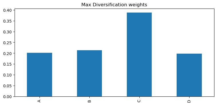
For the example portfolio of investments A, B, C, and D, we can determine the following weights—first as the closed-form solution from formula (7), with the budget constraint as the only constraint.
Compared with the strategies above, it is striking that the MD approach invests considerably more in asset C than in asset B, even though C is substantially riskier. This is due to C’s low correlations with the other investments.
These weights produce the weighted variance-covariance matrix shown in the following table.
The weighted variance-covariance matrix gives an MD portfolio variance of 0.009076, corresponding to a portfolio return standard deviation of 9.52681%:
\[\sigma_p=\sqrt{0.009076}=9.52681\%.\]
As with the risk parity approach, we can tabulate the MD portfolio’s absolute risk contributions (RC), relative risk contributions, the covariances of each investment return with the portfolio return, the beta factors relative to the MD portfolio, and the marginal risk contributions:
Code
# calculation of the absolute risk contribution: formulas (1) and (2)rc=np.zeros(4)for i inrange(4): rc[i]=(weight_md[i]*Sigma[i,:]*np.asmatrix(weight_md).T)/0.0952681# calculation of the relative risk contributionrrc=np.zeros(4)for i inrange(4): rrc[i]=rc[i]/np.sum(rc)# calculation of the covariance of the asset return with the portfolio return: formula (3)cov_ri_rp=np.zeros(4)for i inrange(4): cov_ri_rp[i]=Sigma[i,:]*np.asmatrix(weight_md).T# calculation of the beta of the asset return with the portfolio returnbeta_ri=np.zeros(4)for i inrange(4): beta_ri[i]=cov_ri_rp[i]/0.0952681**2# and now the marginal risk contributionmrc=np.zeros(4)for i inrange(4): mrc[i]=rc[i]/weight_md[i]# Finally we present the results for the MD strategy# clearly in a tableresults_md=pd.DataFrame({'absolute RC (%)': np.round(rc*100,4), \'relative RC (%)': np.round(rrc*100,4),'Cov(r_i,r_p)':np.round(cov_ri_rp,4),'Beta': np.round(beta_ri,4),'MRC (%)': np.round(mrc*100,4)},index=Assets) results_md.loc['Total', results_md.columns[:2]] = results_md.iloc[:, :2].sum(axis=0)results_md
absolute RC (%)
relative RC (%)
Cov(r_i,r_p)
Beta
MRC (%)
A
2.0418
21.4317
0.0097
1.0641
10.1375
B
1.3219
13.8754
0.0059
0.6503
6.1952
C
3.4941
36.6770
0.0086
0.9459
9.0111
D
2.6690
28.0159
0.0129
1.4188
13.5167
Total
9.5268
100.0000
NaN
NaN
NaN
For the MD portfolio, the diversification ratio is:
The diversification ratio can be increased through either its numerator or its denominator: adding riskier investments raises the numerator, while combining investments so as to minimize total risk lowers the denominator. What matters is the gap between the sum of the individual risks and the combined total risk, which is to be maximized and in which the correlations among the investments play a central role. The name “maximum-diversification portfolio” can nonetheless be misleading, since the same set of investments may allow other portfolios with lower total risk.
If all investments in the MD portfolio have the same standard deviation, the numerator of the diversification ratio satisfies:
\[ \Sigma^N_{n=1}w_n\cdot \sigma_n=\sigma_n \quad \textrm{(where for all investments i and j in the portfolio it holds that:} \quad \sigma_i=\sigma_j). \]
In that case the DR is maximized when \(\sigma_p\) is minimized, so the MD and GMV portfolios coincide. Similarly, in the special case where all correlations between the investments are identical, the MD portfolio coincides with the ERC and ERB portfolios.
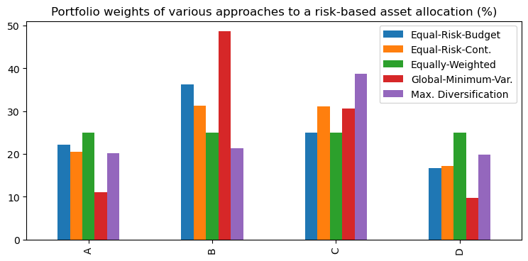
7.5.6 Comparative analysis of the five approaches
We start with a summary of the five weight vectors determined above, first as a table
pd.DataFrame((np.vstack((weight_erb, weight_erc, weight_ew, weight_gmv,\ weight_md))*100).T, index=Assets,\columns = ['Equal-Risk-Budget','Equal-Risk-Cont.','Equally-Weighted',\'Global-Minimum-Var.', 'Max. Diversification']). \ plot.bar(title='Portfolio weights of various approaches to a risk-based asset allocation (%)', legend=True, figsize=(9, 4));
Equally-weighted approach (EW approach)
In the EW approach, the asset weights are set without reference to any expected or statistical quantities. The portfolio structure depends only on the number of investments, all of which receive the same weight. If the weights are reset to \(1/N\) at regular intervals, a security that has performed comparatively well since the last rebalancing is scaled back down to \(1/N\)—so gains are realized at that point.
In terms of weights, the EW approach produces the least concentrated portfolio. When the investments’ risks differ widely, however, the resulting risk concentration means the EW portfolio realizes correspondingly little diversification benefit. Under the strict assumptions of equal expected returns, equal standard deviations, and uniform correlations across the investments, the EW portfolio is nonetheless efficient in the portfolio-theoretic sense (cf. Maillard et al., 2009, p. 2; Demey et al., 2010, p. 12).
Global-minimum-variance approach (GMV approach)
The GMV portfolio is essentially the only portfolio on the efficient frontier whose composition does not depend on expected returns. Like the EW approach, it is easy to understand, and it has the further advantage of a low standard deviation—at least on an ex-ante basis. Its drawback is that it diversifies with respect to standard deviation but not with respect to the individual weights, so it can often end up concentrated in relatively few investments (cf. Demey et al., 2010, p. 12).
As shown, the GMV approach produces marginal risk contributions that are identical across all investments. Thus—again on an ex-ante basis—an infinitesimal increase in any investment’s weight would raise total portfolio risk by the same amount.
Maximum-diversification approach (MD approach)
The MD approach identifies the portfolio with the highest diversification ratio (DR). As with the other approaches in this analysis, it requires no estimate of expected returns. The goal is to maximize the ratio of the portfolio risk without diversification to the (actual) portfolio risk with diversification. For the example portfolio used in the previous sections, the approaches yield the following diversification ratios:
\[DR_{EW}=1.69221368\]
\[DR_{ERB}=1.70560573\]
\[DR_{ERC}=1.75228375\]
\[DR_{GMV}=1.64746376\]
\[DR_{MD}=1.77558125\]
Risk parity approach
By contrast, the risk parity approach seeks to equalize either the risk budget (ERB approach) or the risk contribution (ERC approach) across all investments. Here we use the standard deviation as the risk measure. (The ERC approach can also be adapted to other risk measures; see Maillard et al., 2009, p. 3.) The ERB approach ignores the correlations between investments—or, equivalently, assumes they are all identical—and gives an investment a higher (lower) weight the lower (higher) its standard deviation. In the ERC approach, by contrast, an investment’s weight is inversely proportional to its beta relative to the ERC portfolio: the lower (higher) the beta, the higher (lower) the weight. As a result, the ERC approach tends to favor investments with a relatively low standard deviation and a relatively low correlation with the ERC portfolio.
Formally, the core principles of the individual approaches developed in the previous sections can be summarized as follows:
Note that for the GMV and ERC approaches, applying the formulas given here to compute a weight \(w_n\) requires already knowing the portfolio being constructed.
One can show that, ex ante, the portfolios’ standard deviations are ordered as follows (cf. Roncalli, 2014, p. 174): \(\sigma_{GMV}\leq \sigma_{ERB} \leq \sigma_{EW}\) or \(\sigma_{GMV}\leq \sigma_{ERC} \leq \sigma_{EW}.\) Comparing the ERB and ERC portfolios is inconclusive, since \(\sigma_{ERB}\) may be larger than, equal to, or smaller than \(\sigma_{ERC}\). For the maximum-diversification portfolio, \(\sigma_{GMV}\leq \sigma_{MD}\) also holds, but comparisons with the ERC and ERB standard deviations are again inconclusive.
Moreover, under the EW, ERB, and ERC approaches (long-only), every investment appears in the portfolio, i.e. \(w_n>0\). Under the GMV and MD approaches, by contrast, some investments may be excluded, i.e. \(w_n\) can equal zero—here too assuming a long-only strategy, so that negative weights (short sales) are ruled out.
If the correlations among the individual investments—and hence between each investment and the portfolio—are all identical, the ERC approach yields the same weights as the ERB and MD approaches. In addition, the MD and GMV portfolios coincide when all investments have equal standard deviations (cf. Roncalli, 2014, p. 174; Choueifaty and Coignard, 2008, p. 43); in that case the EW and ERB portfolios also coincide.
The ERC and GMV portfolios coincide when the correlations between the investments are equal and, in addition, approach the limiting value (cf. Maillard et al., 2009, p. 8 and p. 21):
\[ Corr(r_i, r_j)=\frac{-1}{N-1}.\]
At exactly this correlation, the portfolio variance implied by the weighted variance-covariance matrix reaches its lowest possible value (zero)—which is also the minimum-variance value, i.e. that of the GMV portfolio. Hence, at this special correlation value, the GMV and ERC portfolios have identical weights.
As for the expected return-to-risk trade-off, portfolio theory says that only a combination of the risk-free asset and the market portfolio (shown in the earlier GMVP figure) is sensible, since every other portfolio is less efficient. This combination gives the (ex-ante) steepest capital market line and hence the (ex-ante) maximum Sharpe ratio. Accounting for both risk and return, then, asset allocation can be framed as maximizing the Sharpe ratio:
One can show that the ERC portfolio is the maximum-Sharpe-ratio portfolio when the investments have identical correlations and identical Sharpe ratios (cf. Roncalli, 2014, p. 123 ff.). For the MD approach, when all investments share the same Sharpe ratio, the diversification ratio is proportional to the Sharpe ratio, so maximizing the diversification ratio is then equivalent to maximizing the Sharpe ratio. In this special case the MD portfolio coincides with the maximum-Sharpe-ratio portfolio—the market portfolio of capital market theory (cf. Choueifaty and Coignard, 2008, p. 41; Roncalli, 2014, p. 171). The MD portfolio therefore has the highest Sharpe ratio only in the special case where all included investments have identical Sharpe ratios. The Sharpe ratio itself, however, plays no part in determining the individual weights, since the risk-return profile is not considered.
Finally, note that in all of these approaches the volatilities and correlations used to determine the weights are forecasts of future values. When they are estimated from historical data, they need not match the values that actually materialize in future periods.
7.6 Summary
In this chapter you have learned the core idea behind risk-based portfolio approaches and why they deliberately avoid explicitly estimating expected returns. You can classify alternative approaches—such as minimum-variance, equal-risk-contribution, and diversification-based strategies—in technical terms and explain their objectives in quantitative portfolio management. You can also use Python to compute risk and covariance measures from historical return data and use them as key inputs, and you have seen how to implement risk-based portfolios in practice and compare their properties systematically. With this foundation, you can critically assess the strengths and weaknesses of risk-based portfolio approaches and give a well-founded rationale for their use in professional portfolio and risk management.
7.7 Further reading and references
Choueifaty, Y., Coignard, Y. (2008). Toward maximum diversification. Journal of Portfolio Management (Fall 2008), pp. 40–51.
Choueifaty, Y., Froidure, T., Reynier, J. (2013). Properties of the most diversified portfolio. Journal of Investment Strategies 2 (Spring 2013), pp. 49-70.
Clarke, R., de Silva, H., Thorley, S. (2006). Minimum-variance portfolios in the U.S. equity market. Journal of Portfolio Management (Fall 2006), pp. 1-14.
Clarke, R., de Silva, H., Thorley, S. (2011). Minimum-variance portfolio composition. Journal of Portfolio Management (Winter 2011), pp. 31-45.
Demey, P., Maillard, S., Roncalli, T. (2010). Risk-based indexation. Working paper.
Kleeberg, J.M. (1995). Der Anlageerfolg des Minimum-Varianz-Portfolios, Bad Soden.
Kleeberg, J.M. (2002). Internationale Minimum-Varianz-Strategien. In: Kleeberg, J.M. & Rehkugler, H. (Hrsg.): Handbuch Portfoliomanagement, 2. Auflage, Bad Soden/Ts., pp. 361-382.
Maillard, S., Roncalli, T., Teiletche, J. (2009). On the properties of equally-weighted risk contributions portfolios. Working paper, Mai 2009.
Roncalli, T. (2014). Introduction to risk parity and budgeting, Boca Ration, Florida.
Go deeper
Experience this chapter in the live seminar
In the in-house seminar Quant Portfolio Management, you will work through these methods hands-on in Python — with personal feedback, tailored case studies, and direct exchange with Prof. Dr. Thomas Mählmann.