4  Improved Estimation of the Input Parameters: Shrinkage Estimators

Source

4.1 Learning Objectives

After completing this chapter, you will be able to …

• explain the purpose of shrinkage estimators in quantitative portfolio management and assess their significance for stabilizing expected-value and covariance estimates.

• describe the basic functioning of shrinkage methods, in particular the principle of combining empirical estimates with structured target values.

• distinguish shrinkage estimators for expected returns and covariance matrices, both computationally and conceptually, from classical sample estimators.

• interpret shrinkage parameters and evaluate their influence on risk and return estimates in the context of portfolio optimization.

• apply shrinkage estimators in a targeted way to derive more robust input parameters for quantitative portfolio decisions.

4.2 Introduction and motivation

One obvious way to address the estimation-error problem concerns a step left open in Markowitz’s original study: finding improved estimators for the input parameters \(\mu\) and \(\Sigma\). The underlying difficulty is that the assumptions about the future values of these parameters are always estimates and are therefore subject to uncertainty. The goal of better estimation procedures is thus to reduce the impact of the estimation-error problem through a more accurate estimation of the parameters.

At first glance it seems surprising that one can find a better estimator for \(\mu\) than the arithmetic mean, which is, after all, the best unbiased estimator when returns are normally distributed. Yet there is room for improvement: unlike the arithmetic mean, one can estimate the expected return of stock i using not only the time series of stock i but also information from the other stocks. Economically, this is not surprising — the arithmetic mean estimates the expected return of BASF solely from BASF’s past returns, whereas the so-called shrinkage estimators, for example, additionally draw on the time series of Bayer stock. The result is a vector of expected returns computed as a weighted average of the arithmetic means and an exogenous estimate (the so-called prior). In essence, the simple, history-based estimates — which are inherently uncertain — are shrunk toward a predefined prior.

The following sections present the three best-known shrinkage estimators used in portfolio optimization: the James-Stein estimator and the Bayes-Stein estimator for the vector of future expected returns \(\mu\), and the Ledoit-Wolf estimator for the future covariance matrix \(\Sigma\).

4.3 James-Stein estimator for \(\mu\)

In the James-Stein (1961) method, the average of the mean returns of all securities in the sample serves as the prior (also called the “grand mean”). The individual means are adjusted — shrunk — toward this grand mean by the amount of the estimated shrinkage factor \(\hat{w}\): the further a sample mean lies from the grand mean, the more strongly it is shrunk. This dampens the influence of extreme values in the sample, which improves the robustness of the estimator and, in turn, reduces the sensitivity of the portfolio. The mathematical formulation below essentially follows Jorion (1986, pp. 283 ff.).

The James-Stein estimator is defined as:

\[ (1) \quad \hat{\mu}_{JS}=(1-\hat{w})Y+\hat{w}Y_0\iota .\]

Here \(\iota\) is the unit vector of dimension \(Nx1\), and \(Y^T=(\bar{r}_1, ..., \bar{r}_N)\) is the row vector of the \(N\) historical return means. \(\bar{r}_i\) is the mean (at time \(t\)) of the returns of security \(i\), based on a time series of \(k\) observations:

\[ (2) \quad \bar{r}_i=\frac{1}{k}\sum_{j=t-k}^{t}r_{i,j} .\]

The prior, in the form of the grand mean, is:

\[ (3) \quad Y_0=\frac{1}{N}\sum_{i}^{N}\bar{r}_{i} . \]

The shrinkage factor \(\hat{w}\) is computed as:

\[ (4) \quad \hat{w}=\min(1, \frac{N-2}{k(Y-Y_0\iota)^T\Sigma^{-1}(Y-Y_0\iota)}). \]

The shrinkage factor ranges from zero to one. The closer the weight \(\hat{w}\) is to 1, the more strongly the sample means are shrunk toward the average return of all securities. Equation (4) shows that the shrinkage factor depends on the total number (\(k\)) of observations in the estimation period, the number (\(N\)) of securities, the covariance matrix \(\Sigma\), and the distance between the individual historical mean returns and the average return of all securities.

The weighting factor \(\hat{w}\) governs how strongly time-series information and exogenous information shape the estimate of the expected returns. With a long observation period (large \(k\)), the time-series information carries more weight, i.e. \(\hat{w}\) is small. Conversely, the prior gains influence the more closely the true expected returns cluster around the (uniform) estimate \(Y_0\). Equation (1) shows that the improvement comes from incorporating the prior: the James-Stein approach thus prevents extreme estimates of expected returns by implicitly smoothing them toward the prior.

4.4 Bayes-Stein estimator for \(\mu\)

As a further shrinkage estimator, Jorion (1986) developed the Bayes-Stein estimator, which likewise shrinks the individual sample means toward a global mean. Unlike the James-Stein estimator, however, it takes the expected return of the minimum-variance portfolio (MVP) as the global mean, while the shrinkage process itself is the same as for James-Stein. Choosing the MVP is justified by the fact that determining the MVP weights requires no assumptions about the expected returns — they depend only on the covariance matrix. If the budget constraint is the only constraint in the optimization, the MVP weight vector can be determined analytically (cf. e.g. Franzen and Schäfer, 2018, pp. 188 f.):

\[ (5) \quad w_{MVP}=\frac{\iota^T\Sigma^{-1}}{\iota^T\Sigma^{-1}\iota}. \]

Assuming that estimation errors in the risk terms (variances and covariances) can be neglected, the MVP is therefore less affected by estimation error. For the expected return of the MVP as the prior it then follows (with \(Y\) as the \(Nx1\) column vector of the empirical return means):

\[ (6) \quad \hat{\mu}_{MVP}=w_{MVP}Y=\frac{\iota^T\Sigma^{-1}Y}{\iota^T\Sigma^{-1}\iota}. \]

The Bayes-Stein estimator is given by:

\[ (7) \quad \hat{\mu}_{BS}=(1-\hat{w})Y+\hat{w}\hat{\mu}_{MVP}\iota . \]

The shrinkage factor by which the individual empirical returns are adjusted toward the MVP return is:

\[ (8) \quad \hat{w}=\frac{N+2}{(N+2)+k(Y-\hat{\mu}_{MVP}\iota)^T\Sigma^{-1}(Y-\hat{\mu}_{MVP}\iota)}, \]

where \(N\) is the number of securities in the portfolio and \(k\) the number of periods in the sample. Besides adjusting the expected returns, Jorion proposes — because the true \(\Sigma\) is unknown — adjusting the estimate of the covariance matrix following Zellner and Chetty (1965), with \(\hat{\Sigma}\) as the empirically estimated covariance matrix (Jorion, 1986, p. 286):

\[ (9) \quad \hat{\Sigma}_{ZC}=\frac{k-1}{k-N-2}\hat{\Sigma} . \]

In an earlier study of the effects of the estimation-error problem on portfolio selection, Jorion (1985) had already found that shrinkage estimators dominate the conventional empirical means in out-of-sample performance. Jorion (1986) then further demonstrated the superiority of the Bayes-Stein estimator over the classical approach.

4.5 Ledoit-Wolf estimator for \(\Sigma\)

Ledoit and Wolf (2003) address the problem of estimating covariance matrices from a sample and propose shrinking the empirical covariance matrix toward a matrix with a fixed structure. Since the number of covariances to be estimated grows quadratically with the number \(N\) of securities (number of covariances \(=0.5\cdot N(N-1)\)), the estimation-error problem becomes more acute when determining the covariance matrix for large portfolios.

The fundamental principle in the shrinkage of the covariance matrix comprises the combination of the following elements:

• empirical covariance matrix \(\hat{\Sigma}\) from the sample without a fixed structure
• shrinkage factor \(\hat{w}\)
• covariance matrix with a fixed structure \(\hat{\Sigma}_{cc}\)

A convex-linear combination (via the shrinkage factor) of the two matrices strikes a compromise between the sample covariance matrix \(\hat{\Sigma}\) and a prescribed fixed structure \(\hat{\Sigma}_{cc}\), the shrinkage target. The shrinkage target should meet two criteria: it should have only a few free parameters, giving the estimator a fixed structure, and it should still capture important features of the unknown parameters being estimated. For the matrix \(\hat{\Sigma}_{cc}\), Ledoit and Wolf (2003) propose either estimating the return correlations from the single-index model of Sharpe (1963) or assuming constant pairwise correlations. Since the latter is easier to implement and generally gives comparable results, we use it in what follows to determine \(\hat{\Sigma}_{cc}\).

This convex-linear combination of the two matrices is:

\[ (10) \quad \hat{\Sigma}_{LW}=\hat{w}\hat{\Sigma}_{cc}+(1-\hat{w})\hat{\Sigma},\]

where \(\hat{\Sigma}\) is the sample covariance matrix and \(\hat{\Sigma}_{cc}\) the sample covariance matrix under the assumption of a constant correlation (cc).

The latter is computed in stages. Since the covariance \(Cov(X,Y)\) of two random variables \(X\) and \(Y\) can be written as the product of the volatilities (\(\sigma_X, \sigma_Y\)) and the correlation coefficient \(Corr(X,Y)\) (i.e. \(Cov(X,Y)=\sigma_X \cdot \sigma_Y \cdot Corr(X,Y)\)), the empirical covariance matrix satisfies:

\[ (11) \quad \hat{\Sigma}=\Lambda C \Lambda^T, \]

where \(\Lambda\) is a diagonal matrix of the return volatilities and \(C\) the sample correlation matrix. With \(\hat{\rho}_{ij}\) the empirical correlation coefficient between the returns of securities \(i\) and \(j\), \(C\) is:

\[ (12)\quad C=\left( \begin{array}{rrrr} 1 & \hat{\rho}_{12} & \dots & \hat{\rho}_{1N} \\ \hat{\rho}_{21} & \ddots & \ddots & \vdots \\ \vdots & \ddots & \ddots & \hat{\rho}_{N-1N} \\ \hat{\rho}_{N1} & \dots & \hat{\rho}_{NN-1} & 1 \\ \end{array}\right) .\]

To compute \(\hat{\Sigma}_{cc}\), the sample correlation matrix is simply replaced by one with constant correlations

\[ (13)\quad C_{cc}=\left( \begin{array}{rrrr} 1 & \hat{\rho} & \dots & \hat{\rho} \\ \hat{\rho} & \ddots & \ddots & \vdots \\ \vdots & \ddots & \ddots & \hat{\rho} \\ \hat{\rho} & \dots & \hat{\rho} & 1 \\ \end{array}\right) ,\]

where \(\hat{\rho}\) is the average of all (\(0.5 \cdot N(N-1)\)) sample correlations. It is given by:

\[ (14) \quad \hat{\rho}=\frac{2}{(N-1)N}\sum_{i=1}^N \sum_{j=i+1}^N \hat{\rho}_{ij} . \]

The shrinkage target is therefore: \(\hat{\Sigma}_{cc}=\Lambda C_{cc} \Lambda^T\)

According to Ledoit and Wolf (2003), the optimal shrinkage factor is the constant that minimizes the expected distance between the shrinkage estimator and the true covariance matrix. It can be shown that the optimal shrinkage intensity is proportional to a constant \(\hat{g}\) divided by the sample size \(k\). The optimal shrinkage factor is therefore:

\[ (15) \quad \hat{w}= max \left \{0, min \left \{\frac{\hat{g}}{k},1\right \} \right \}. \]

The following case study illustrates the calculation of the three shrinkage estimators and their effects on the composition of optimal portfolios.

4.6 Start of the case study

We begin by importing the required packages.

import pandas as pd
import numpy as np
from scipy.optimize import minimize
import matplotlib.pyplot as plt
import numpy.linalg as la

4.6.1 Loading and describing the data

The data set contains price histories (beginning-of-month prices) for the following ten companies: Abbott Laboratories (ABT), Boeing Industries (BA), Costco Wholesale (COST), Cisco Systems (CSCO), IBM (IBM), Intel (INTC), Merk (MRK), Microsoft (MSFT), AT&T (T), and Exxon Mobil Corporation (XOM). The prices cover the period 12.2004-12.2009 (61 months).

# insert here your local directory path of the file
# cd "..."

frame = pd.read_excel('Kapitel A1.xlsx', 'Tabelle1', index_col=0, parse_dates=True)

frame.tail(6)

	ABT	BA	COST	CSCO	IBM	INTC	MRK	MSFT	T	XOM
2009-07-01	44.99	42.91	49.50	22.01	117.93	19.25	30.01	23.52	26.23	70.39
2009-08-03	45.23	49.67	50.98	21.60	118.05	20.32	32.43	24.65	26.05	69.15
2009-09-01	49.47	54.15	56.38	23.54	119.61	19.57	31.63	25.72	27.01	68.61
2009-10-01	50.57	47.80	56.85	22.81	120.61	19.11	30.93	27.73	25.67	71.67
2009-11-02	54.49	52.41	59.91	23.40	126.35	19.20	36.21	29.41	26.94	75.07
2009-12-01	54.48	53.72	60.73	23.92	127.94	19.66	36.88	30.01	27.18	76.04

From continuous (log) returns, we compute and annualize the historical means and the covariance matrix of the returns.

# using log returns
log_returns = np.log1p(frame.pct_change().dropna()) 
means = log_returns.mean().values*12 # annualised
Sigma = log_returns.cov().values*12 # annualised

4.6.2 James-Stein estimator

We now compute the grand mean \(Y_0\), the shrinkage factor \(\hat{w}\), and the James-Stein expected returns \(\hat{\mu}_{JS}\) using formulas (1), (3), and (4) above.

# overall average return = return prior for James-Stein
grand_mean=np.mean(means)

# James-Stein shrinkage factor
phi_js = np.min([1,(len(means)-2)/(len(log_returns)*(np.matrix(means-grand_mean)*\
        la.inv(Sigma)*np.matrix(means-grand_mean).T)[0,0])])

# James-Stein expected returns
js_means = (1-phi_js)*means + phi_js*grand_mean

phi_js

0.4475110828261736

For the present data, formula (4) gives a shrinkage factor of \(\hat{w}=0.44\). Using this factor, the James-Stein estimator then yields the expected returns of the individual securities. A comparison with the conventionally estimated expected returns gives:

pd.DataFrame({'JS-Means (%)': np.round(js_means, 4)*100,\
              'Hist. Means (%)': np.round(means,4)*100,\
             'Abs. Difference (%)': np.round(js_means-means, 4)*100},\
             index=frame.columns)

	JS-Means (%)	Hist. Means (%)	Abs. Difference (%)
ABT	2.99	3.10	-0.12
BA	1.68	0.74	0.94
COST	3.78	4.53	-0.76
CSCO	3.63	4.27	-0.64
IBM	4.15	5.21	-1.06
INTC	-0.65	-3.47	2.83
MRK	2.79	2.75	0.04
MSFT	2.55	2.32	0.23
T	1.86	1.07	0.79
XOM	5.63	7.89	-2.26

Or, as a bar chart:

pd.DataFrame({'JS-Means': js_means, 'Hist. Means': means},index=frame.columns). \
plot.bar(stacked=False, alpha=0.5, figsize=(10,5));

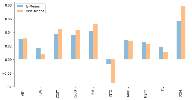
The differences between the conventional expected-return estimates and the James-Stein forecasts turn out to be small. But given that classical portfolio optimization already reacts very sensitively to small deviations in the expected returns, the influence of the James-Stein estimator on the optimization should not be underestimated.

4.6.3 Bayes-Stein estimator

First we compute the adjusted covariance-matrix estimator \(\hat{\Sigma}\) following Zellner and Chetty (1965). The adjustment factor is \(\frac{k-1}{k-N-2}\) (see formula (9) above).

adj_Sigma = ((len(log_returns)-1)/(len(log_returns)-len(means)-2))*Sigma

With the budget constraint as the only constraint, the MVP weights are: \[ (5) \quad w_{MVP}=\frac{\iota^T\Sigma^{-1}}{\iota^T\Sigma^{-1}\iota}. \]

iota = np.ones(Sigma.shape[0]) # identity vector of dimension 10
inv_adj_Sigma = la.inv(adj_Sigma)
Weight_GMV = inv_adj_Sigma @ iota / (iota @ inv_adj_Sigma @ iota)
pd.DataFrame([round(x,4) for x in Weight_GMV],index=frame.columns).T

	ABT	BA	COST	CSCO	IBM	INTC	MRK	MSFT	T	XOM
0	0.4359	-0.0418	0.2083	-0.0125	0.141	0.0902	-0.1451	-0.0239	0.0445	0.3035

The expected return of the MVP, from equation (6): \(\hat{\mu}_{MVP}=w_{MVP}Y\).

# expected return of MVP (= return prior for James-Stein)
eret_GMV = (np.matrix(Weight_GMV)* np.matrix(means).T)[0,0]
eret_GMV

0.0462098479530484

The BS shrinkage factor, from equation (8):

\[ (8) \quad \hat{w}=\frac{N+2}{(N+2)+k(Y-\hat{\mu}_{MVP}\iota)^T\Sigma^{-1}(Y-\hat{\mu}_{MVP}\iota)}. \]

# calculation of Bayes-Stein shrinkage factor phi_bs:
phi_bs = (len(means)+2)/((len(means)+2) + len(log_returns)*(np.matrix(means-eret_GMV)\
        * inv_adj_Sigma * np.matrix(means-eret_GMV).T)[0,0])
phi_bs

0.4777796219708953

This gives a shrinkage factor of \(\hat{w}=0.48\). The Bayes-Stein estimator of the expected returns is then:

\[ \quad \hat{\mu}_{BS}=(1-\hat{w})Y+\hat{w}\hat{\mu}_{MVP}\iota . \]

# Bayes-Stein expected returns
bs_means = (1-phi_bs)*means + phi_bs*eret_GMV

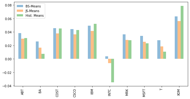
A comparison of the three estimators (JS, BS, Historical) of \(\mu\), in table form:

pd.DataFrame({'JS-Means': np.round(js_means,4),\
              'BS-Means': np.round(bs_means,4),\
              'Hist. Means': np.round(means,4)},\
             index=frame.columns)

	JS-Means	BS-Means	Hist. Means
ABT	0.0299	0.0383	0.0310
BA	0.0168	0.0259	0.0074
COST	0.0378	0.0458	0.0453
CSCO	0.0363	0.0444	0.0427
IBM	0.0415	0.0493	0.0521
INTC	-0.0065	0.0039	-0.0347
MRK	0.0279	0.0364	0.0275
MSFT	0.0255	0.0342	0.0232
T	0.0186	0.0276	0.0107
XOM	0.0563	0.0633	0.0789

or as a bar chart:

pd.DataFrame({'BS-Means': bs_means, 'JS-Means': js_means, 'Hist. Means': means},index=frame.columns). \
plot.bar(stacked=False, alpha=0.5, figsize=(10,5));

4.6.4 Ledoit-Wolf estimator of the covariance matrix

Via log_returns.corr().values we compute the empirical correlation matrix \(C\) from the continuous returns and store it in the array corr. The average correlation \(\hat{\rho}\) is obtained with mean(corr[corr!=1]), where the condition corr!=1 excludes the diagonal elements \(\hat{\rho}_{ii}\) of \(C\).

corr = log_returns.corr().values
Sigma = log_returns.cov().values*12

# average of pairwise correlation (without diagonal elements)
avg_corr = np.mean(corr[corr!=1])

Construction of the correlation matrix \(C_{cc}\) with constant correlation

np.eye(len(corr)) generates an \(NxN\) diagonal matrix with zeros off the diagonal and ones on the main diagonal, and np.ones((len(corr), len(corr))) an \(NxN\) “ones” matrix. Multiplying the two by (1-avg_corr) and avg_corr respectively and adding them gives \(C_{cc}\).

# generating a corr matrix with constant correlations as off diagonal
constant_corr = \
(1-avg_corr)*np.eye(len(corr)) + avg_corr*np.ones((len(corr), len(corr)))

Construction of the covariance matrix \(\hat{\Sigma}_{cc}\) under the assumption of constant correlation

The following holds: \(\hat{\Sigma}_{cc}=\Lambda C_{cc} \Lambda^T\).

Via np.sqrt(np.diagonal(Sigma)) we extract the diagonal elements (variances) of the empirical covariance matrix \(\hat{\Sigma}\) into an array of volatilities, which np.diag() then turns into the diagonal matrix \(\Lambda\).

# calculation of covariance matrix using a constant correlation assumption 
# the first part is diagonal matrix containing the volatilities p.a.
const_Sigma =\
(np.diag(np.sqrt(np.diagonal(Sigma))).dot(constant_corr)).dot(  \
 np.diag(np.sqrt(np.diagonal(Sigma))))

Assuming a shrinkage factor of \(\hat{w}=0.45\), we can now determine the Ledoit-Wolf estimator of the covariance matrix from equation (10):

\[ (10) \quad \hat{\Sigma}_{LW}=\hat{w}\hat{\Sigma}_{cc}+(1-\hat{w})\hat{\Sigma}.\]

# assuming a given shrinkage constant phi_lw
phi_lw = 0.45

# calculating the Ledoit-Wolf covariance matrix
lw_Sigma = phi_lw * const_Sigma + (1-phi_lw)*Sigma

lw_Sigma.shape

(10, 10)

4.6.5 Comparison of the efficient frontiers and portfolio allocations

4.6.5.1 General

Once the expected returns (and the covariance matrix) have been determined, they can enter the portfolio optimization as inputs. In what follows we consider the case with the long-only constraint (implemented via positive holding limits).

First we define the optimization’s target functions (\(\sigma_P^2 \rightarrow \min_{w}!\) or, for the MRP, \(\mu_P \rightarrow \max_{w}!\)) and determine the weights of the minimum-variance portfolio (MVP) and the maximum-return portfolio (MRP). The MVP’s composition does not depend on the estimate of the expected-return vector. Running the optimization for various target returns between the MVP and MRP returns then traces out the corresponding efficient frontier.

# definition of target function for MVP to be minimized
def calculate_portfolio_var(w,Sigma):
    # function that calculates portfolio risk
    w = np.matrix(w) # w is a row (not column!) vector
    return (w*Sigma*w.T)[0,0]

# definition of target function for MRP to be maximized
def calculate_negative_portfolio_ret(w,means):
    # function that calculates -1 times the portfolio expected return
    w = np.matrix(w) # w is a row (not column!) vector
    means = np.matrix(means)
    return -(w*means.T)[0,0]

def calculate_portfolio_ret(w,means):
    # function that calculates portfolio expected return
    w = np.matrix(w) # w is a row (not column!) vector
    means = np.matrix(means)
    return (w*means.T)[0,0]

Weights of the MVP and the MRP (using the historical covariance matrix Sigma and the long-only constraint, with the naive portfolio as starting weights).

# use equal weights "Weight_1N" as starting values 
Weight_1N = np.tile(1.0/means.shape[0], means.shape[0])

# positive weight portfolio
bnd=[(0, 1),(0, 1),(0, 1),(0, 1),(0, 1),
     (0, 1),(0, 1),(0, 1),(0, 1),(0, 1)] # only positive weights
cons = ({'type': 'eq', 'fun': lambda x:  np.sum(x)-1.0})

# MVP
res2= minimize(calculate_portfolio_var, Weight_1N, args=Sigma, 
               bounds = bnd, method='SLSQP',constraints=cons,tol=1e-10, 
               options={'disp': True})
Weight_MV2 = res2.x

# MRP
res4= minimize(calculate_negative_portfolio_ret, Weight_1N, args=means, 
               bounds = bnd, method='SLSQP',constraints=cons,tol=1e-10, 
               options={'disp': True})
Weight_MRP = res4.x

Optimization terminated successfully    (Exit mode 0)
            Current function value: 0.012112846573987465
            Iterations: 21
            Function evaluations: 231
            Gradient evaluations: 21
Optimization terminated successfully    (Exit mode 0)
            Current function value: -0.07886975933686077
            Iterations: 11
            Function evaluations: 121
            Gradient evaluations: 11

4.6.5.2 James-Stein versus historical means

First we determine the range of target returns, separately for the JS and the historically estimated expected returns.

# calculation of min and max target return
# min: expected return of MVP, max: expected return of MRP

# for historic means
min = calculate_portfolio_ret(Weight_MV2, means)
max = calculate_portfolio_ret(Weight_MRP, means)

# for JS means
min_js = calculate_portfolio_ret(Weight_MV2, js_means)
max_js = calculate_portfolio_ret(Weight_MRP, js_means)

We now compute the efficient frontiers, first for the historical means:

# efficient frontier with hist. mean returns
V_Target = np.linspace(min, max, num=45)
V_Risk = np.zeros(V_Target.shape)
V_Return = np.zeros(V_Target.shape)
V_Weight = np.zeros((V_Target.shape[0], means.shape[0]))
for idx, Target_Return in enumerate(V_Target):
    cons = ({'type': 'eq', 'fun': lambda x:  np.sum(x)-1.0},
            {'type': 'eq', 'fun': lambda x:  calculate_portfolio_ret(x,means)-Target_Return})
    res= minimize(calculate_portfolio_var, Weight_1N, args=Sigma, 
               bounds = bnd, method='SLSQP',constraints=cons,tol=1e-10)
    V_Weight[idx, :] = res.x.T
    V_Return[idx] = calculate_portfolio_ret(res.x,means)
    V_Risk[idx] = np.sqrt(calculate_portfolio_var(res.x, Sigma))

And now for the JS expected returns:

# efficient frontier with JS mean returns
V_Target_js = np.linspace(min_js, max_js, num=45)
V_Risk_js = np.zeros(V_Target.shape)
V_Return_js = np.zeros(V_Target.shape)
V_Weight_js = np.zeros((V_Target.shape[0], means.shape[0]))
for idx, Target_Return in enumerate(V_Target_js):
    cons = ({'type': 'eq', 'fun': lambda x:  np.sum(x)-1.0},
            {'type': 'eq', 'fun': lambda x:  calculate_portfolio_ret(x,js_means)-Target_Return})
    res= minimize(calculate_portfolio_var, Weight_1N, args=Sigma, 
               bounds = bnd, method='SLSQP',constraints=cons,tol=1e-10)
    V_Weight_js[idx, :] = res.x.T
    V_Return_js[idx] = calculate_portfolio_ret(res.x,js_means)
    V_Risk_js[idx] = np.sqrt(calculate_portfolio_var(res.x, Sigma))

Plot of the efficient frontiers:

fig1 = plt.figure(num=1, facecolor='w', figsize=(10, 5))
ax = fig1.add_subplot(111)
plt.plot(V_Risk, V_Target, 'g:', label='Hist.-efficient frontier without short selling')
plt.plot(V_Risk_js, V_Target_js, 'g-', label='JS-efficient frontier without short selling')
plt.plot(np.sqrt(np.diagonal(Sigma)), means, 'rx', label='Asset')
for i, txt in enumerate(frame.columns):
   ax.annotate(txt, (np.sqrt(np.diagonal(Sigma))[i],means[i]))
plt.legend(loc=3,  frameon=True)
plt.xlabel('Standard deviation')
plt.ylabel('Expected return')
plt.title('Comparing efficient frontiers')
plt.show()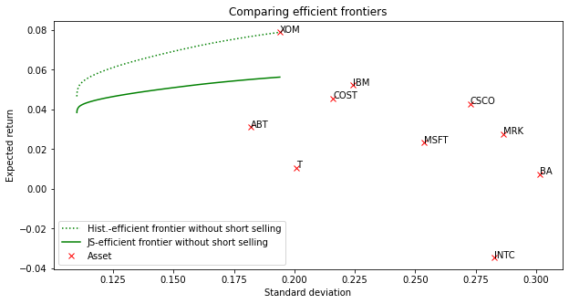

The efficient frontier based on the James-Stein expected returns clearly lies below the conventional one, even though the absolute differences between the two estimation methods were only minor.

If, however, the portfolio weights along the entire efficient frontier are shown together in an area chart, it is striking at first glance how little the weights seem to differ. On closer inspection, though, the weights have shifted along the horizontal axis, and the expected returns have been reassigned accordingly.

Portfolio weights based on the historically estimated expected returns:

fig2 = plt.figure(num=2, facecolor='w', figsize=(10, 5))
plt.stackplot(V_Target, V_Weight.T*100)
plt.axis([min, max, 0.0, 100.0])
plt.legend(list(frame.columns),
           loc='upper left', bbox_to_anchor=(1.0, 1.0), frameon=False)
plt.xlabel('Target expected return (%)')
plt.ylabel('Allocation weight (%)')
plt.title('Portfolioweights based on historic mean returns')
plt.show()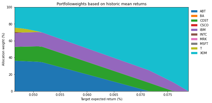

Portfolio weights based on the JS estimator of the expected returns:

fig3 = plt.figure(num=2, facecolor='w', figsize=(10, 5))
plt.stackplot(V_Target_js, V_Weight_js.T*100)
plt.axis([min_js, max_js, 0.0, 100.0])
plt.legend(list(frame.columns),
           loc='upper left', bbox_to_anchor=(1.0, 1.0), frameon=False)
plt.xlabel('Target expected return') 
plt.title('Portfolioweights based on JS mean return estimates')
plt.ylabel('Allocation weight (%)')
plt.show()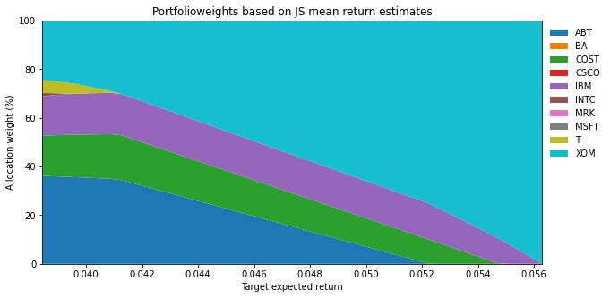

4.6.5.3 Bayes-Stein versus historical means

We determine the range of target returns for the efficient frontier based on the BS estimator of the expected returns.

# calculation of min and max target return
# min: expected return of MVP, max: expected return of MRP

min_bs = calculate_portfolio_ret(Weight_MV2, bs_means)
max_bs = calculate_portfolio_ret(Weight_MRP, bs_means)

Calculation of the efficient frontier:

V_Target_bs = np.linspace(min_bs, max_bs, num=45)
V_Risk_bs = np.zeros(V_Target.shape)
V_Return_bs = np.zeros(V_Target.shape)
V_Weight_bs = np.zeros((V_Target.shape[0], means.shape[0]))
for idx, Target_Return in enumerate(V_Target_bs):
    cons = ({'type': 'eq', 'fun': lambda x:  np.sum(x)-1.0},
            {'type': 'eq', 'fun': lambda x:  calculate_portfolio_ret(x,bs_means)-Target_Return})
    res= minimize(calculate_portfolio_var, Weight_1N, args=Sigma, 
               bounds = bnd, method='SLSQP',constraints=cons,tol=1e-10)
    V_Weight_bs[idx, :] = res.x.T
    V_Return_bs[idx] = calculate_portfolio_ret(res.x,bs_means)
    V_Risk_bs[idx] = np.sqrt(calculate_portfolio_var(res.x, Sigma))

Graphical representation:

fig4 = plt.figure(num=1, facecolor='w', figsize=(10, 5))
ax = fig4.add_subplot(111)
plt.plot(V_Risk, V_Target, 'g:', label='Hist.-efficient frontier without short selling')
plt.plot(V_Risk_bs, V_Target_bs, 'g--', label='BS-efficient frontier without short selling')
plt.plot(np.sqrt(np.diagonal(Sigma)), means, 'rx', label='Asset')
for i, txt in enumerate(frame.columns):
   ax.annotate(txt, (np.sqrt(np.diagonal(Sigma))[i],means[i]))
plt.legend(loc=3,  frameon=True)
plt.xlabel('Standard deviation')
plt.ylabel('Expected return')
plt.title('Comparing efficient frontiers')
plt.show();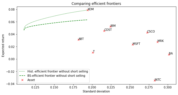

The efficient frontier of the Bayes-Stein estimator lies below the conventional one. As with the James-Stein estimator, if the portfolio weights along the entire efficient frontier are shown together in an area chart, it is striking at first glance how little the weights appear to differ. On closer inspection, though, the weights have indeed shifted along the horizontal axis, and the expected returns have likewise been reassigned.

Portfolio weights based on the BS estimator of the expected returns:

fig5 = plt.figure(num=2, facecolor='w', figsize=(10, 5))
plt.stackplot(V_Target_bs, V_Weight_bs.T*100)
plt.axis([min_bs, max_bs, 0.0, 100.0])
plt.legend(list(frame.columns),
           loc='upper left', bbox_to_anchor=(1.0, 1.0), frameon=False)
plt.xlabel('Target expected return') 
plt.title('Portfolioweights based on BS mean return estimates')
plt.ylabel('Allocation weight (%)')
plt.show()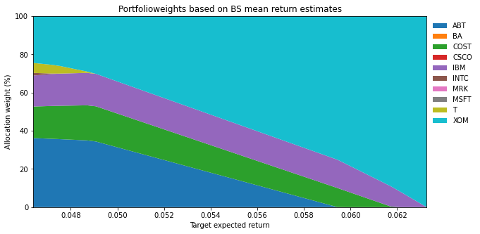

4.6.5.4 Ledoit-Wolf versus historically estimated covariance matrix

We compute the weights of the minimum-variance portfolio based on the Ledoit-Wolf estimate of the covariance matrix.

bnd=[(0, 1),(0, 1),(0, 1),(0, 1),(0, 1),
     (0, 1),(0, 1),(0, 1),(0, 1),(0, 1)] # only positive weights
cons = ({'type': 'eq', 'fun': lambda x:  np.sum(x)-1.0})

res2= minimize(calculate_portfolio_var, Weight_1N, args=lw_Sigma, 
               bounds = bnd, method='SLSQP',constraints=cons,tol=1e-10, 
               options={'disp': True})
Weight_MV2_lw = res2.x

Optimization terminated successfully    (Exit mode 0)
            Current function value: 0.014806352991309255
            Iterations: 22
            Function evaluations: 242
            Gradient evaluations: 22

We determine the range of target returns (using the historical means as the estimator of \(\mu\)).

# calculation of min and max target return
# min: expected return of MVP, max: expected return of MRP

min_lw = calculate_portfolio_ret(Weight_MV2_lw, means)
max_lw = calculate_portfolio_ret(Weight_MRP, means) # no change here!

Calculation of the efficient frontier.

V_Target_lw = np.linspace(min_lw, max_lw, num=45)
V_Risk_lw = np.zeros(V_Target.shape)
V_Return_lw = np.zeros(V_Target.shape)
V_Weight_lw = np.zeros((V_Target.shape[0], means.shape[0]))
for idx, Target_Return in enumerate(V_Target_lw):
    cons = ({'type': 'eq', 'fun': lambda x:  np.sum(x)-1.0},
            {'type': 'eq', 'fun': lambda x:  calculate_portfolio_ret(x,means)-Target_Return})
    res= minimize(calculate_portfolio_var, Weight_1N, args=lw_Sigma, 
               bounds = bnd, method='SLSQP',constraints=cons,tol=1e-10)
    V_Weight_lw[idx, :] = res.x.T
    V_Return_lw[idx] = calculate_portfolio_ret(res.x,means)
    V_Risk_lw[idx] = np.sqrt(calculate_portfolio_var(res.x, lw_Sigma))

Plot of the efficient frontier based on the Ledoit-Wolf covariance matrix versus the historically estimated one.

fig6 = plt.figure(num=1, facecolor='w', figsize=(10, 5))
ax = fig6.add_subplot(111)
plt.plot(V_Risk, V_Target, 'g:', label='Hist.-efficient frontier without short selling')
plt.plot(V_Risk_lw, V_Target_lw, 'g-', label='LW-efficient frontier without short selling')
plt.plot(np.sqrt(np.diagonal(Sigma)), means, 'rx', label='Asset')
for i, txt in enumerate(frame.columns):
   ax.annotate(txt, (np.sqrt(np.diagonal(Sigma))[i],means[i]))
plt.legend(loc='best',  frameon=True)
plt.xlabel('Standard deviation')
plt.ylabel('Expected return')
plt.title('Comparison of efficient frontiers')
plt.show()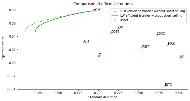

Portfolio weights based on the Ledoit-Wolf estimator of the covariance matrix:

fig7 = plt.figure(num=2, facecolor='w', figsize=(10, 5))
plt.stackplot(V_Target_lw, V_Weight_lw.T*100)
plt.axis([min_lw, max_lw, 0.0, 100.0])
plt.legend(list(frame.columns),
           loc='upper left', bbox_to_anchor=(1.0, 1.0), frameon=False)
plt.xlabel('Target expected return') 
plt.title('Portfolioweights based on LW covariance estimates')
plt.ylabel('Allocation weight (%)')
plt.show()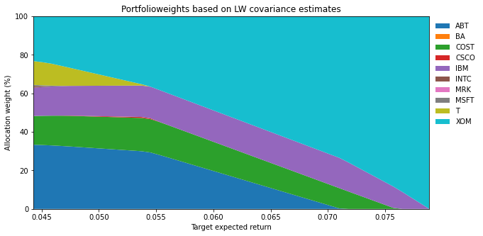

4.7 Summary

In this chapter you have met the purpose of shrinkage estimators in quantitative portfolio management and understood their significance for stabilizing estimates of expected values and covariances. You can explain how shrinkage methods work and how empirical estimates are combined with structured target values. You are also able to distinguish shrinkage estimators, both conceptually and computationally, from classical sample estimators. You have learned to interpret shrinkage parameters and to assess their influence on risk and return estimates in the optimization. This equips you to apply shrinkage estimators in a targeted way to derive more robust input parameters for quantitative portfolio decisions.

4.8 Literature and references

• Franzen, D., Schäfer, K. (2018). Assetmanagement. Schäffer-Poeschel, Stuttgart.
  
• James, W., Stein, C. (1961). Estimation with quadratic loss. In Proceedings of the fourth Berkeley symposium on mathematical statistics and probability.
  
• Jorion, P. (1985). International portfolio diversification with estimation risk. Journal of Business 58, pp. 259-278.
  
• Jorion, P. (1986). Bayes-Stein estimation for portfolio analysis. Journal of Financial and Quantitative Analysis 21, pp. 279-292.
  
• Ledoit, O., Wolf, M. (2003). Improved estimation of the covariance matrix of stock returns with an application to portfolio selection. Journal of Empirical Finance 10, pp. 603-621.
  
• Sharpe, W. (1963). A simplified model for portfolio analysis. Management Science 9, pp. 277-293.
  
• Zellner, A., Chetty, V. K. (1965). Prediction and decision problems in regression models from the Bayesian point of view. Journal of the American Statistical Association 60, pp. 608-616.

Go deeper

Experience this chapter in the live seminar

In the in-house seminar Quant Portfolio Management, you will work through these methods hands-on in Python — with personal feedback, tailored case studies, and direct exchange with Prof. Dr. Thomas Mählmann.

Learn more about the seminar →