3 Estimation Risks in Portfolio Theory

3.1 Learning Objectives
After completing this chapter, you will be able to …
explain the concept of estimation risk in portfolio theory and describe its causes, particularly in the estimation of expected returns and covariances from historical data.
analyze how estimation errors affect the results of classical portfolio optimization and can lead to unstable or economically implausible portfolio weights.
describe typical methods for reducing estimation risk, e.g., shrinkage methods (robust estimators) or simplified model assumptions.
handle estimation risk in practice in Python, use suitable libraries, and soundly assess optimization results while accounting for the uncertainty in the input data.
3.2 Introduction and motivation
The following presentation is based on:
- Kempf, A./Memmel, C. Schätzrisiken in der Portfoliotheorie. In: Kleeberg, J.M. & Rehkugler, H. (eds.): Handbuch Portfoliomanagement, 2. Auflage, Bad Soden/Ts. 2002, pp. 895-919.
- Memmel, C. Schätzrisiken in der Portfoliotheorie: Auswirkungen und Möglichkeiten der Reduktion, Eul Verlag, Lohmar, 2004.
In his groundbreaking 1952 Journal of Finance article “Portfolio Selection”, Harry Markowitz argues that risk-averse investors should base their decisions on the expected value and variance of their overall portfolio’s return. The investor seeks to achieve a given expected portfolio return at the lowest possible risk. Formalizing this idea mathematically leads to a quadratic optimization problem with N-1 decision variables, where N is the number of admissible investment instruments.
Implementing Markowitz’s approach in practice comes with a central problem: the investor does not know the parameters of the return distributions (expected values, variances, covariances). These parameters can be determined, for example, from fundamental company data or — as we will focus on here — estimated from historical time series. For large portfolios, this estimation is first of all a challenge of sheer quantity, since N expected returns and variances, plus 0.5 · N · (N-1) covariances, must be estimated. Even for an investment universe of just 500 stocks, that already amounts to 125,750 parameters. Beyond this quantity problem, however, there is a second, more serious one, which will be the focus of what follows. Every estimate carries an estimation risk: the estimated parameter will generally not match the (unobservable) true parameter of the return distribution. This can lead to suboptimal portfolios and hence to poor investment outcomes. The aim of this chapter is to show how important estimation risk is for portfolio composition, and then to present ways of reducing its influence.
3.3 Influence of the estimation error on portfolio composition
First, a small simulation study illustrates how strongly estimation risk affects portfolio composition. To this end, we simulate independent, identically normally distributed weekly returns for four stocks over a two-year period. For each stock we assume an expected return of 11% p.a. and a standard deviation of 25% p.a., and we assume that the returns of the different stocks have a pairwise correlation of 0.3. We also assume a risk-free instrument with a return of \(r_f\) = 6% p.a. We include this risk-free instrument so that the optimal composition of the stock portfolio is independent of the investor’s degree of risk aversion (Tobin separation). Tobin (1958) showed that in this case all investors hold the same stock portfolio — the so-called tangency portfolio — regardless of their risk aversion.
To gauge the magnitude of the estimation risks, we examine the optimal composition of an investor’s tangency portfolio in two cases: in the first, the investor knows the distribution parameters above; in the second, they must estimate them from the simulated return realizations. If the investor knows the parameters, the optimum is to spread the wealth invested in stocks evenly across the four stocks. This equal-weighting strategy yields an expected stock-portfolio return of 11% p.a. with a standard deviation of 17.23% p.a. We now turn to the case in which the investor estimates the parameters from the realized returns.
Starting situation for the simulation:
true parameters (annualized): \(\mu_i=0.11, \sigma_i=0.25, \rho_{ij}=0.3\), for \(i,j =1,..., 4,\) and \(i \neq j\).
The variance at the weekly level is: \(0.25^{2}/52=0.00120192\).
For the weekly expected return: \(0.11/52=0.00211538\).
The constant correlation coefficient is 0.3. This gives the weekly covariance: \(0.25^{2}/52 * 0.3=0.00036058\).
Code
# We call the weekly variance-covariance matrix *Sigma_true*:
Sigma_true=[[0.00120192, 0.00036058, 0.00036058, 0.00036058],\
            [0.00036058, 0.00120192, 0.00036058, 0.00036058],\
            [0.00036058, 0.00036058, 0.00120192, 0.00036058],\
            [0.00036058, 0.00036058, 0.00036058, 0.00120192]]

# The vector of expected weekly returns:
means_true=[0.00211538, 0.00211538, 0.00211538, 0.00211538]
Code
# a Monte Carlo draw, each with a 2-year time series
# (104 weeks) for each stock
np.random.seed(42)
df = pd.DataFrame(np.asarray(np.random.multivariate_normal(means_true,\
                Sigma_true, size = 104)), columns=['A1', 'A2', 'A3', 'A4'])
means_est = df.mean().values * 52 # annualized
Sigma_est = df.cov().values * 52 # annualized
std_est=np.sqrt(np.diag(Sigma_est))
The next two tables show the estimated parameters for one example random path of the simulation alongside the true values. First, a comparison of the true and estimated expected returns:
Code
| true | estimated | Estimation error (%) | |
|---|---|---|---|
| A1 | 0.11 | 0.193280 | -8.328017 |
| A2 | 0.11 | 0.179376 | -6.937638 |
| A3 | 0.11 | 0.086520 | 2.347950 |
| A4 | 0.11 | 0.192972 | -8.297215 |
And now the comparison of the true (0.25) and estimated standard deviations:
Code
| true | estimated | Estimation error (%) | |
|---|---|---|---|
| A1 | 0.25 | 0.233158 | 1.684243 |
| A2 | 0.25 | 0.239306 | 1.069351 |
| A3 | 0.25 | 0.231460 | 1.854000 |
| A4 | 0.25 | 0.231680 | 1.831986 |
Let us now compute the optimal weights of the tangency portfolio, i.e. the portfolio with the maximum Sharpe ratio. We impose only the budget constraint: no leverage (borrowing), so that the portfolio weights sum to 1.
Code
# function that implements the Sharpe portfolio optimization
# with no short sale constraint!

# definition of target function for maximum Sharpe portfolio
def calc_neg_sharpe(weights, mean_returns, cov, rf):
    portfolio_return = np.sum(mean_returns * weights)
    portfolio_std = np.sqrt(np.dot(weights.T, np.dot(cov, weights)))
    sharpe_ratio = (portfolio_return - rf) / portfolio_std
    return -sharpe_ratio

def max_sharpe_ratio(mean_returns, cov, rf):
    num_assets = len(mean_returns)
    args = (mean_returns, cov, rf)
    constraints = ({'type': 'eq', 'fun': lambda x: np.sum(x) - 1})
    result = minimize(calc_neg_sharpe, num_assets*[1./num_assets,], args=args,
                        method='SLSQP', constraints=constraints,tol=1e-10)
    weights=[round(x,4) for x in result['x']]
return weightsA graphical comparison of the optimal portfolio weights: the true weights (1/N) versus those obtained from the estimated input parameters:
Code
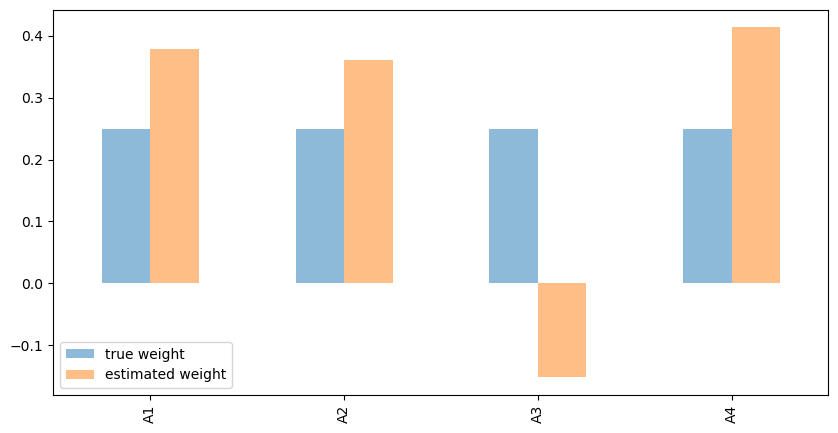
Two results stand out. First, the optimal weights based on the estimated parameters differ dramatically from the true optimal values — estimation errors clearly have a serious impact on portfolio composition. Second, the estimates of the expected return deviate far more from their true value than the estimates of the standard deviation, which stay much closer to the true parameter. This is a first sign that estimating the expected return is where the greatest difficulty lies — a point we pursue further in the next section.
3.4 Components of the estimation error
So far, we have examined how the total estimation error affects portfolio composition, without asking which source of the error (misestimated expected returns, variances, or correlations) has the strongest impact on the portfolio weights. That impact depends on two things: the sensitivity of the portfolio composition to the misestimation, and the size of the misestimation. In what follows, we first analyze the sensitivity of the portfolio composition to the various components of the estimation error, and then discuss how accurately each parameter can actually be estimated.
3.4.1 Sensitivity of the optimal portfolio with respect to estimation errors in the various parameters
To analyze how sensitive the portfolio weights are to misestimations of the individual parameters, we again use the four stocks from Section 1, with true parameters \(\mu_i\) = 11% (expected return), \(\sigma_i\) = 25% (standard deviation), and \(\rho_{ij}\) = 30% (correlation coefficient). As a benchmark, we take the case in which the investor knows all parameters exactly, so that the optimal stock portfolio consists of equal shares in all four stocks. This is compared with three cases in which the investor makes an estimation error in the parameters of stock 1: in the first, about the expected return of stock 1; in the second, about its standard deviation; and in the third, about the correlation between the returns of stock 1 and stock 2. The individual cases used to determine the components of estimation risk are shown in the following table.
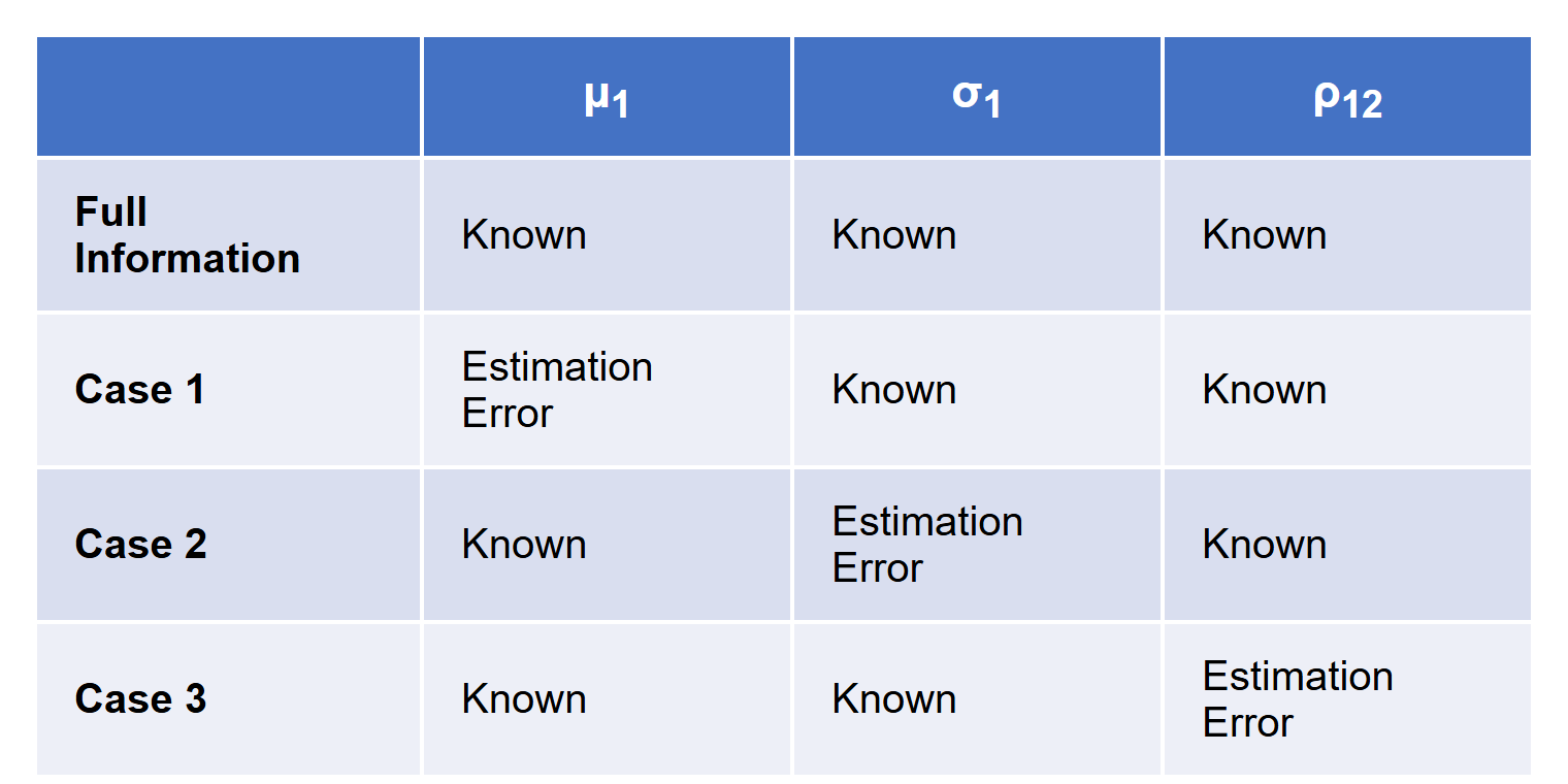
We examine the influence of the estimation error in a comparative-static analysis, varying the mis-estimated parameter around its true value by ±10 percentage points in steps of 2.0 percentage points. The expected return thus ranges from 1% to 21%, the volatility from 15% to 35%, and the correlation from 20% to 40%. For each parameter combination, we determine the optimal portfolio composition and compare it with the optimal composition obtained when all parameters are known.
Case 1: Estimation error in the expected return of stock 1, between 1% and 21% around the true value of 11%.
Code
# calculation of the misweighting in A1 for errors in the estimated
# expected return
est_error_mean=np.linspace(0.01, 0.21, 11) # symmetric errors around the true value 11%
wa1_means=np.zeros(11) # contains the optimized weights
for i in range(11):
    means_mod=np.multiply(means_true,52) # do not forget to annualize!
    Sigma_true_ann=np.multiply(Sigma_true,52) # do not forget to annualize!
    means_mod[0]=est_error_mean[i]
    weights=max_sharpe_ratio(means_mod, Sigma_true_ann, 0.06)
    wa1_means[i]=weights[0]
Case 2: Estimation error in the standard deviation of the return of stock 1, between 15% and 35% around the true value of 25%.
Code
# calculation of the misweighting in A1 for errors in the estimated
# (annualized) standard deviation
est_error_std=np.linspace(0.15, 0.35, 11) # symmetric errors around the true value 25%
# calculation of the new variance and covariance
a1_var=np.zeros(11) # contains the new variance
a1_cov=np.zeros(11) # contains the new covariance
wa1_std=np.zeros(11) # contains the optimized weights

for i in range(11):
    a1_var[i]=est_error_std[i]**2
    a1_cov[i]=est_error_std[i]*0.25*0.3
    # calculation of the new variance-covariance matrix; make 7 changes
    Sigma_true_ann=np.multiply(Sigma_true,52) # do not forget to annualize!
    Sigma_mod=Sigma_true_ann
    Sigma_mod[0,0]=a1_var[i]
    Sigma_mod[0,1]=a1_cov[i]
    Sigma_mod[0,2]=a1_cov[i]
    Sigma_mod[0,3]=a1_cov[i]
    Sigma_mod[1,0]=a1_cov[i]
    Sigma_mod[2,0]=a1_cov[i]
    Sigma_mod[3,0]=a1_cov[i]
    means_ann=np.multiply(means_true,52) # do not forget to annualize!
    weights=max_sharpe_ratio(means_ann, Sigma_mod, 0.06)
    wa1_std[i]=weights[0]
Case 3: Estimation error in the correlation of the return of stock 1, between 20% and 40% around the true value of 30%.
Code
# calculation of the misweighting in A1 for errors in the estimated
# correlation between stock 1 and 2
est_error_corr=np.linspace(0.20, 0.40, 11) # symmetric errors around the true value 25%
# calculation of the new covariance
a1_cov=np.zeros(11) # contains the new covariance
wa1_corr=np.zeros(11) # contains the optimized weights

for i in range(11):
    a1_cov[i]=est_error_corr[i]*0.25*0.25
    # calculation of the new variance-covariance matrix; make 2 changes
    Sigma_true_ann=np.multiply(Sigma_true,52) # do not forget to annualize!
    Sigma_mod=Sigma_true_ann
    Sigma_mod[0,1]=a1_cov[i]
    Sigma_mod[1,0]=a1_cov[i]
    means_ann=np.multiply(means_true,52) # do not forget to annualize!
    weights=max_sharpe_ratio(means_ann, Sigma_mod, 0.06)
    wa1_corr[i]=weights[0]
The following table gives the optimal weight of stock 1 in the various cases.
Code
| Deviations from the true parameter value in (%) | -10.0 | -8.0 | -6.0 | -4.0 | -2.0 | 0.0 | 2.0 | 4.0 | 6.0 | 8.0 | 10.0 |
|---|---|---|---|---|---|---|---|---|---|---|---|
| Case 1 | -1.79 | -1.11 | -0.62 | -0.26 | 0.02 | 0.25 | 0.44 | 0.59 | 0.72 | 0.83 | 0.93 |
| Case 2 | 0.66 | 0.56 | 0.47 | 0.38 | 0.31 | 0.25 | 0.20 | 0.16 | 0.12 | 0.09 | 0.07 |
| Case 3 | 0.27 | 0.27 | 0.26 | 0.26 | 0.25 | 0.25 | 0.25 | 0.24 | 0.24 | 0.24 | 0.23 |
The table clearly shows that changes in the expected return have the strongest impact on portfolio composition. If, for example, the expected return of stock 1 is overestimated by 6 percentage points, the optimal weight of stock 1 becomes 0.72 — an overweighting of 47 percentage points relative to the error-free optimum. A misestimation of the standard deviation of the same size has a much weaker effect (-0.13 = 0.12 - 0.25), and a misestimation of the correlation has no notable effect at all (-0.01 = 0.24 - 0.25). The following figure illustrates this once more, plotting the over- or under-weighting of stock 1 against the size of the estimation error.
Code
fig1 = plt.figure(num=1, facecolor='w', figsize=(10, 5))
ax = fig1.add_subplot(111)
ax.spines['left'].set_position('zero')
ax.spines['right'].set_position('zero')
ax.spines['top'].set_position('zero')

ax.spines['bottom'].set_position('zero')
plt.plot(np.linspace(-10, 10, 11), (wa1_means-0.25)*100, 'r-', label='Error in the expected return')
plt.plot(np.linspace(-10, 10, 11), (wa1_std-0.25)*100, 'g-', label='Error in the standard deviation')
plt.plot(np.linspace(-10, 10, 11), (wa1_corr-0.25)*100, 'b-', label='Error in the correlation coefficient')

plt.legend(loc=4,  frameon=True)
plt.xlabel('Magnitude of the misestimation (in %)')
ax.yaxis.set_label_coords(-0.01,0.75)
ax.xaxis.set_label_coords(0.5,-0.01)

plt.ylabel('Misweighting in stock 1 (in %)')
plt.title('Effect of estimation errors on the optimal weights in stock 1')
plt.show()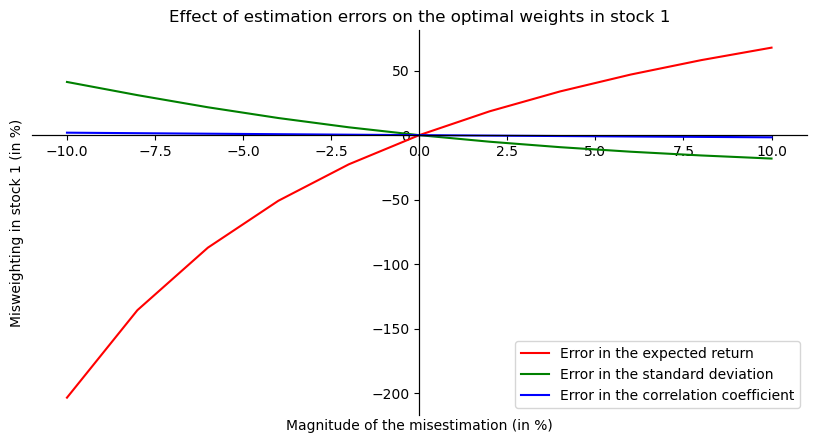
The figure clearly shows that even small errors in the parameter estimates cause substantial changes in the optimized weights — especially errors in the expected returns. The sensitivity of the portfolio composition to estimation errors is thus a central problem in applying Markowitz’s approach. How strongly an investor is affected, however, depends not only on this sensitivity but also on how accurately each parameter can be estimated. We analyze that estimation accuracy next.
3.4.2 Magnitude of the estimation errors for the various parameters
From historical data, we want the most reliable possible estimates of the expected annualized return \((\mu_i)\) and the annualized standard deviation \((\sigma_i)\). (We omit the correlation here, since — as noted above — the portfolio composition is very insensitive to misestimations of the correlation.) For this, a time series of n (non-annualized) period returns \(r_{t,i}\) is available, assumed to be independent, identically, and normally distributed, with expected value \(\mu_i\Delta t\) and variance \(\sigma^2_i\Delta t\). To reduce the estimation error, the investor tries to increase the number of observations entering the estimate — either by extending the estimation period \(T\) (in years) or by splitting it into shorter subintervals, i.e. by shortening \(\Delta t\).
For various reasons, however, an investor often cannot extend the observation period \(T\). Young companies have no long price history. Others do, but it is marked by breaks caused by restructurings or acquisitions. And a long price history is questionable anyway, because the return parameters do not stay constant over decades. The investor has more freedom, by contrast, in choosing the length of the subintervals: they can move from annual to quarterly, monthly, weekly, daily, or even intraday data to increase the number of observations. In what follows, we examine how this affects the quality of the estimators of the expected return and the variance. First we must assume which estimator the investor uses; again we assume simple history-based estimation, i.e. the arithmetic mean for the first moment. Using the fact that the estimation period \(T\) equals the number of subperiods n times their length \(\Delta t\), the mean estimator can be written as:
\[ (1)\quad \hat{\mu_i}=\frac{1}{\Delta t}\frac{1}{n}\sum_{t=1}^{n}r_{t,i}=\frac{1}{T}\sum_{t=1}^{n}r_{t,i}.\]
This estimator is unbiased, i.e. on average it hits the true parameter value \(\mu_i\). Its quality is measured by its variance: the smaller the variance, the less the estimator scatters around the true value. The estimator’s variance is:
\[ (2)\quad var(\hat{\mu_i})=\frac{\sigma^2_i}{T}.\]
Remarkably, for a fixed observation period \(T\) this quality measure does not depend on the data frequency: increasing the sampling frequency does not make the estimate any more accurate. It is also striking how large the estimation error is relative to the quantity being estimated. This is easiest to see using the data from our example in Section 1, where a stock has an expected return of 11% p.a. and a return standard deviation of 25% p.a. The following table shows the width of a 95% confidence interval as a function of the estimation-period length \(T\). In general, the width of the (asymptotic) \((1-\alpha)\) confidence interval is:
\[ (3)\quad 2\cdot[Q_{1-\frac{\alpha}{2}}\cdot\frac{\sigma_i}{\sqrt{T}}].\]
Here \(Q_{1-\frac{\alpha}{2}}\) is the \((1-\frac{\alpha}{2})\) quantile of the standard normal distribution. For \(\alpha=5\%\): \(Q_{97.5}=1.96\)
Code
# length of the estimation period T in years
est_period=[1, 5, 10, 20, 50]
# width of the confidence interval
confidence=np.zeros(5)
for i in range(5):
    confidence[i]=round((2*1.96*0.25/np.sqrt(est_period[i]))*100, 2)
pd.DataFrame({'Estimation period T in years': est_period, \
'Width of the confidence interval (%)': confidence}) | Estimation period T in years | Width of the confidence interval (%) | |
|---|---|---|
| 0 | 1 | 98.00 |
| 1 | 5 | 43.83 |
| 2 | 10 | 30.99 |
| 3 | 20 | 21.91 |
| 4 | 50 | 13.86 |
Even with an estimation period of 10 years, this interval is still more than 30 percentage points wide. In other words, with 95% probability the estimation error is no larger than 15.5 percentage points, i.e. the estimate lies in the interval [-4.5%;+26.5%]. Yet, as shown above, even a much smaller misestimation has a dramatic effect on portfolio composition.
We now turn to the variance estimate. Using the definitional relationship \(T = n \cdot \Delta t\), the simple history-based estimator can be written as:
\[ (4)\quad \hat{\sigma}^2_i=\frac{1}{T-\Delta t}\sum_{t=1}^{n}(r_{t,i}-\hat{\mu_i}\Delta t)^2.\]
The asymptotic variance of this estimator is (see Memmel, 2004, p. 33):
\[ (5)\quad var(\hat{\sigma}^2_i)=\frac{2\sigma^4_i\Delta t}{T}.\]
So, for a given estimation period \(T\), the variance estimator can be improved by increasing the data frequency (reducing \(\Delta t\)). Switching from quarterly to monthly data, for example, triples the number of observations and cuts the estimation error to roughly a third of its original value.
The asymptotic variance of the estimator of the return standard deviation is:
\[ (6)\quad var(\hat{\sigma}_i)=\frac{1}{2}\sigma^2_i\frac{\Delta t}{T}.\]
The following table lists the widths of the 95% confidence interval (in %) for the estimator of the annualized-return standard deviation, for various estimation-period lengths and data frequencies.
Code
# length of the estimation period T in years
est_period=[1, 5, 10, 20, 50]
# width of the confidence interval
confidence_daily=np.zeros(5) # delta_t=1/250
confidence_weekly=np.zeros(5) # delta_t=1/52
confidence_monthly=np.zeros(5) # delta_t=1/12
confidence_quarterly=np.zeros(5) # delta_t=1/4

for i in range(5):
    confidence_daily[i]=round(2*1.96*np.sqrt(0.25**2/ \
                    (2*est_period[i]*250))*100, 2)
    confidence_weekly[i]=round(2*1.96*np.sqrt(0.25**2/ \
                    (2*est_period[i]*52))*100, 2)
    confidence_monthly[i]=round(2*1.96*np.sqrt(0.25**2/ \
                    (2*est_period[i]*12))*100, 2)
    confidence_quarterly[i]=round(2*1.96*np.sqrt(0.25**2/ \
                    (2*est_period[i]*4))*100, 2)
Zeitraum=['T=1 year', 'T=5 years', 'T=10 years', 'T=20 years', 'T=50 years']
pd.DataFrame({'Daily data': confidence_daily, 'Weekly data': confidence_weekly,\
              'Monthly data': confidence_monthly, 'Quarterly data': confidence_quarterly},\
index=Zeitraum) | Daily data | Weekly data | Monthly data | Quarterly data | |
|---|---|---|---|---|
| T=1 year | 4.38 | 9.61 | 20.00 | 34.65 |
| T=5 years | 1.96 | 4.30 | 8.95 | 15.50 |
| T=10 years | 1.39 | 3.04 | 6.33 | 10.96 |
| T=20 years | 0.98 | 2.15 | 4.47 | 7.75 |
| T=50 years | 0.62 | 1.36 | 2.83 | 4.90 |
Compared with the previous table, it is striking that the standard deviation can be estimated far more accurately than the expected return — and, all else equal, the more so the higher the data frequency. With daily data, for instance, a fairly precise variance estimate is possible even over a one-year estimation period, whereas over the same period the expected return can be estimated only very imprecisely. The results so far thus seem to suggest that, for a given estimation period, an investor should use the highest possible data frequency, since by (5) this reduces the estimation error in the variance while leaving that in the expected return unchanged. This conclusion, however, needs qualifying. In practice, a very high data frequency means the observed returns are no longer independent, identically, and normally distributed: at high frequencies (e.g. daily data), stock returns exhibit autocorrelation, and their distribution has too much mass in the tails.
In summary: estimating expected returns is considerably more problematic than estimating the return variance. Estimates of expected returns cannot be improved by increasing the data frequency, whereas estimates of the variance can. And since the portfolio composition reacts far more sensitively to misestimated expected returns than to misestimated variances, estimation errors in the expected returns must be regarded as the central problem in implementing the Markowitz model. In what follows, we therefore focus solely on estimation errors in the expected returns and assume that the second moments of the distribution (variances, correlations) are known to the investor.
3.5 Solution approaches for the estimation problem
In the previous sections, we worked out why the traditional implementation of portfolio theory is problematic. With the traditional arithmetic-mean estimator, expected returns can be estimated only very imprecisely, which typically produces extreme and suboptimal portfolio weights.
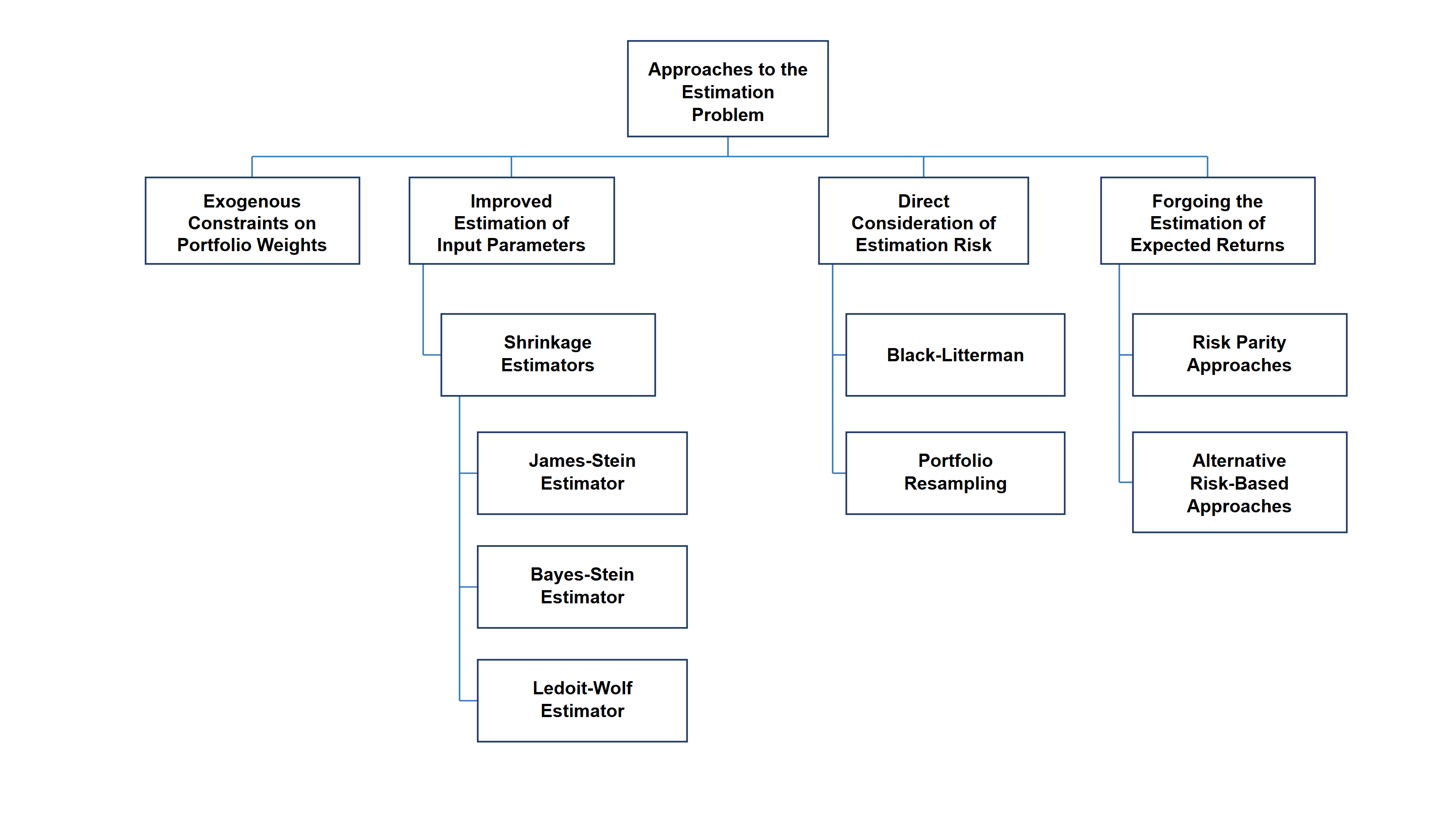
In principle, several options are available. The first is to develop an economically well-founded model in which the optimal portfolio weights arise endogenously and which relies on quantities that are easier to determine than the expected returns. An example is the CAPM, in which the optimal portfolio weights equal the relative market capitalizations.
A second option, aimed at reducing the influence of estimation errors and the extreme weights they produce, is to impose exogenous bounds (constraints) on the expected returns or the portfolio weights. Merton (1980) takes the first route, assuming that, in a world of risk-averse investors, the true expected returns cannot be negative and should not exceed some maximum value. A simple example of exogenous bounds on the portfolio weights — already present in Markowitz’s original work — is the ban on short selling, which restricts each stock’s weight to the range [0%; 100%]. The optimal strategy here often consists of corner solutions: in most cases the capital is concentrated in a few stocks that have performed particularly well recently (a winner strategy). This sacrifices diversification within the portfolio. To remedy this, one limits how far the portfolio weights may deviate from those of an index or benchmark portfolio — for example, within relative (index- or benchmark-based) optimization. This forced but non-optimal diversification does reduce portfolio risk, but at the cost of the portfolio’s performance.
The third option is to dispense with estimating expected returns altogether. An investor could, for example, choose the global minimum-variance stock portfolio or an equally weighted portfolio. Such a portfolio is best described as heuristic, since it does not follow from a general Markowitz approach. Even so, various empirical studies (e.g. DeMiguel et al., 2009) have found that these strategies can outperform the traditional implementation of portfolio theory.
Alongside these classical heuristics, risk-based approaches have become increasingly established since the 2008-2009 financial crisis. These, too, build the portfolio solely from volatility and correlation assumptions, with diversification at the center; forecasts of expected returns play no role and are not needed. Three risk-based construction methods are distinguished — Equal Risk Budget (ERB), Equal Risk Contribution (ERC), and Maximum-Diversification (MD) — of which the first two are known as Risk Parity approaches. All three are methodologically closely related: the aim is always to invest in every asset class at comparable risk, reducing an asset class’s weight as its volatility or its correlation with another asset class rises.
The fourth option for reducing the influence of estimation risk in the expected returns is to improve the estimator of the expected returns and then use this improved estimate as an input to the portfolio optimization. A popular class of such improved estimators, for both \(\mu\) and \(\Sigma\), are the so-called shrinkage estimators.
The fifth option, finally, also uses an improved estimator of the expected returns (as in the fourth option) but additionally accounts for the remaining estimation risk within the portfolio optimization. It thus explicitly recognizes that the investor faces two kinds of risk: return-fluctuation risk and estimation risk. Two well-known representatives are the portfolio resampling method of Michaud and Michaud (2008) and the Black/Litterman (BL) model (see Black and Litterman, 1992).
The following figure once again groups the solution approaches outlined above by their underlying starting points.
3.6 Summary
In this chapter you have met the concept of estimation risk in portfolio theory and understood the causes of the uncertainty in estimating expected returns and covariances. You can analyze how estimation errors affect the results of classical portfolio optimization and lead to unstable or economically implausible portfolio weights. You are also able to describe typical methods for reducing estimation risk, such as shrinkage procedures or simplified model assumptions. And you have learned to handle estimation risk in practice in Python and to assess optimization results soundly, accounting for the uncertainty in the input data.
3.7 Literature and references
- Black, F., Litterman R. (1992). Global Portfolio Optimization. Financial Analysts Journal (September-October), pp. 28-43.
- DeMiguel, V., Garlappi, L., Uppa, R. (2009). Optimal Versus Naive Diversification: How Inefficient is the 1/N Portfolio Strategy? Review of Financial Studies 22, pp. 1915-1953.
- Kempf, A., Memmel, C. (2002). Schätzrisiken in der Portfoliotheorie. In: Kleeberg, J.M., Rehkugler, H. (eds.): Handbuch Portfoliomanagement, 2. Auflage, Bad Soden/Ts. 2002, pp. 895-919.
- Markowitz, H.M. (1952). Portfolio Selection. Journal of Finance 7, pp. 77-91.
- Memmel, C. (2004). Schätzrisiken in der Portfoliotheorie: Auswirkungen und Möglichkeiten der Reduktion. Eul Verlag, Lohmar, 2004.
- Merton, R.C. (1980). On Estimating the Expected Return on the Market: An Exploratory Investigation. Journal of Financial Economics 8, pp. 323-361.
- Michaud, R.O, Michaud, R.O., (2008). Efficient Asset Management: A Practical Guide to Stock Portfolio Optimization and Asset Allocation, 2nd Edition, Oxford University Press.
- Tobin, J. (1958). Liquidity Preference as Behaviour Towards Risk. Review of Economic Studies 25, pp. 65-86.
Go deeper
Experience this chapter in the live seminar
In the in-house seminar Quant Portfolio Management, you will work through these methods hands-on in Python — with personal feedback, tailored case studies, and direct exchange with Prof. Dr. Thomas Mählmann.
Learn more about the seminar →